Generate Krylov time-evolution circuits (SKQD)

Important

The concepts in this guide are currently available only in the Python API. Equivalent functionality will be made available through the C API in a future release.

Sample-based Krylov Quantum Diagonalization (SKQD) is a quantum-centric variant of subspace diagonalization. Rather than sampling a single variational ansatz (as in plain SQD) or an ensemble of randomized time-evolution circuits (as in SqDRIFT), it samples a Krylov basis: the family of states

\[\lvert \psi_k \rangle = e^{-i k \, \Delta t \, H} \lvert \psi_0 \rangle, \qquad k = 0, 1, \dots, D - 1,\]

obtained by evolving a reference state \(\lvert \psi_0 \rangle\) for increasing multiples of a fixed time step \(\Delta t\). Bitstrings sampled from these \(D\) circuits populate the Krylov subspace in which the Hamiltonian is subsequently diagonalized classically.

This guide reproduces the circuit-construction step of the SKQD algorithm for the single-impurity Anderson model (SIAM) – a magnetic impurity coupled to a non-interacting bath – following the SKQD publication.

Note

The SKQD sampling step works only if the ground state is sparse in the computational basis: the classical diagonalization must be able to reconstruct it from a manageable number of sampled bitstrings. As we will see, that sparsity is not automatic – it is a property of the single-particle basis in which the problem is expressed. Getting the basis right is the crux of this construction.

1. Build the SIAM Hamiltonian as a fermionic operator

The single-impurity Anderson model places one interacting impurity orbital (index \(0\)) in contact with a non-interacting bath of \(L\) sites arranged as a chain. Its Hamiltonian splits into a one-body part \(H_1\) and a two-body part \(H_2\),

\[H = H_1 + H_2,\]

with the one-body part collecting the impurity on-site energy (the chemical potential \(\mu\)), the impurity–bath hybridization \(V\), and the nearest-neighbor bath hopping \(t\),

\[H_1 = \mu \sum_\sigma a^\dagger_{0\sigma} a_{0\sigma} - V \sum_\sigma \left( a^\dagger_{0\sigma} a_{1\sigma} + \text{h.c.} \right) - t \sum_{\sigma} \sum_{i=1}^{L-1} \left( a^\dagger_{i\sigma} a_{i+1,\sigma} + \text{h.c.} \right),\]

and the two-body part carrying the on-site Coulomb repulsion \(U\) on the impurity alone,

\[H_2 = U \, a^\dagger_{0\uparrow} a_{0\uparrow} a^\dagger_{0\downarrow} a_{0\downarrow}.\]

We work at the particle-hole-symmetric point \(\mu = -U/2\). These two parts map directly onto the one-body integrals h1e (bath hopping, impurity hybridization, impurity on-site energy) and the single two-body integral h2e (the impurity Coulomb term). We first assemble them in the position basis, where the model is naturally defined.

>>> import numpy as np
>>>
>>> norb = 8
>>> nelec = (norb // 2, norb // 2)  # half filling
>>> hopping, onsite, hybridization = 1.0, 10.0, 1.0
>>> chemical_potential = -0.5 * onsite
>>>
>>> # one-body integrals: bath hopping, impurity hybridization, and impurity on-site energy
>>> h1e = np.zeros((norb, norb))
>>> np.fill_diagonal(h1e[:, 1:], -hopping)
>>> np.fill_diagonal(h1e[1:, :], -hopping)
>>> h1e[0, 1] = h1e[1, 0] = -hybridization
>>> h1e[0, 0] = chemical_potential
>>>
>>> # two-body integrals: on-site Coulomb repulsion on the impurity orbital
>>> h2e = np.zeros((norb,) * 4)
>>> h2e[0, 0, 0, 0] = onsite

2. Change to the momentum basis

The bath part of the SIAM is a free-fermion chain, so it is diagonalized by a change to the momentum basis. This is the decisive step for SKQD: because the bath is translationally invariant, the ground state is not sparse in the position basis, but it is sparse in the momentum basis, where the bath Hamiltonian is diagonal. The single-particle orbital rotation that performs this change is problem-specific linear algebra – it diagonalizes the bath hopping matrix while leaving the impurity orbital untouched, then relocates the impurity to a central site:

>>> def momentum_basis(norb):
...     """Orbital rotation from the position to the momentum basis."""
...     n_bath = norb - 1
...     hopping_matrix = np.zeros((n_bath, n_bath))
...     np.fill_diagonal(hopping_matrix[:, 1:], -1)
...     np.fill_diagonal(hopping_matrix[1:, :], -1)
...     _, vecs = np.linalg.eigh(hopping_matrix)
...     orbital_rotation = np.zeros((norb, norb))
...     orbital_rotation[0, 0] = 1.0
...     orbital_rotation[1:, 1:] = vecs
...     new_index = n_bath // 2
...     perm = np.r_[1:(new_index + 1), 0, (new_index + 1):norb]
...     return orbital_rotation[:, perm]
...
>>> orbital_rotation = momentum_basis(norb)

Unlike a variational workflow, here we rotate the Hamiltonian integrals into the momentum basis, so that the whole circuit – Hamiltonian and state alike – lives in the basis where the ground state is sparse and the sampled bitstrings are therefore informative. Rotating the one- and two-body integrals is a standard basis change of the electronic-structure tensors:

>>> rotation = orbital_rotation.T.conj()
>>> h1e_momentum = np.einsum("ab,Aa,Bb->AB", h1e, rotation, rotation.conj(), optimize="greedy")
>>> h2e_momentum = np.einsum(
...     "abcd,Aa,Bb,Cc,Dd->ABCD",
...     h2e,
...     rotation,
...     rotation.conj(),
...     rotation,
...     rotation.conj(),
...     optimize="greedy",
... )

Because the rotation leaves the impurity orbital fixed (it acts only on the bath), the on-site interaction stays put: h2e_momentum remains a single number-number term, just like h2e – the only change is that the impurity has been relocated to a central index. We can see this directly in the integral tensors, which each carry exactly one nonzero entry:

>>> print(f"h2e nonzero at:          {np.argwhere(np.abs(h2e) > 1e-12).tolist()}")
h2e nonzero at:          [[0, 0, 0, 0]]
>>> print(f"h2e_momentum nonzero at: {np.argwhere(np.abs(h2e_momentum) > 1e-12).tolist()}")
h2e_momentum nonzero at: [[3, 3, 3, 3]]

This locality is what keeps the interaction cheap to synthesize later.

We assemble the one-body integrals into a FermionOperator with the electronic-integral constructor from_1body_tril_spin_sym(), which expects them packed into lower-triangular ordering. The two-body part is a single number-number term, so rather than route it through the two-body integral machinery we build it directly with cre()/ann() – the on-site Coulomb operator \(U \, n_{p\uparrow} n_{p\downarrow}\) for the impurity mode \(p\) (its \(\uparrow\) mode at index p, its \(\downarrow\) mode at index p + norb in the block-spin layout). Both constructors spin-double the norb spatial orbitals into 2 * norb fermionic modes.

We keep the one-body part \(H_1\) and the two-body part \(H_2\) as separate operators rather than summing them eagerly – the terms \(H_1\) and \(H_2\) of the section-1 equations. Building each piece once (in both bases) lets us reuse them below: summed, they give the full Hamiltonian for the exact diagonalization in either basis; individually, \(H_2\) (momentum basis) is exactly the operator the Trotter step evolves in step 4.

>>> from qiskit_fermions.operators import FermionOperator, ann, cre
>>>
>>> # U n_imp_up n_imp_down: the impurity's up/down modes sit at `imp` and `imp + norb` in the
>>> # block-spin layout (the impurity is orbital 0 in the position basis, orbital 3 in the
>>> # momentum basis -- the single relocated index found above)
>>> imp_pos, imp_mom = 0, 3
>>>
>>> one_body_position = FermionOperator.from_1body_tril_spin_sym(
...     h1e[np.tril_indices(norb)], norb
... )
>>> two_body_position = FermionOperator.from_dict(
...     {(cre(imp_pos), ann(imp_pos), cre(imp_pos + norb), ann(imp_pos + norb)): onsite}
... )
>>> one_body_momentum = FermionOperator.from_1body_tril_spin_sym(
...     h1e_momentum[np.tril_indices(norb)], norb
... )
>>> two_body_momentum = FermionOperator.from_dict(
...     {(cre(imp_mom), ann(imp_mom), cre(imp_mom + norb), ann(imp_mom + norb)): onsite}
... )
>>>
>>> hamiltonian_position = (
...     (one_body_position + two_body_position).normal_ordered().simplify(atol=1e-14)
... )
>>> hamiltonian_momentum = (
...     (one_body_momentum + two_body_momentum).normal_ordered().simplify(atol=1e-14)
... )

The basis change is a unitary similarity transform, so it leaves the spectrum untouched: we can confirm the operator is correct by comparing its lowest eigenvalue in the \((\text{norb}, \text{nelec})\) sector against an exact diagonalization. The FermionOperator exposes a SciPy LinearOperator (backed by a native FCI matrix-vector kernel), so we can hand it straight to scipy.sparse.linalg.eigsh().

>>> import scipy.sparse.linalg
>>> from qiskit_fermions.linalg import linear_operator
>>>
>>> linop = linear_operator(hamiltonian_momentum, norb, nelec)
>>> reference_energy, ground_state = scipy.sparse.linalg.eigsh(linop, k=1, which="SA")
>>> reference_energy = reference_energy[0]
>>> ground_state = ground_state[:, 0]
>>> print(f"exact ground-state energy: {reference_energy:.6f}")
exact ground-state energy: -13.422492

The payoff of the basis change is sparsity. To make it concrete, we count how many computational-basis determinants are needed to capture 99% of the ground-state weight – and compare the momentum basis against the position basis. The energy is basis-independent, but the number of determinants is not:

>>> def determinants_for(vec, fraction=0.99):
...     weights = np.sort(np.abs(vec) ** 2)[::-1]
...     return int(np.searchsorted(np.cumsum(weights), fraction) + 1)
...
>>> # the same Hamiltonian in the position basis has an identical spectrum, but a dense ground state
>>> position_linop = linear_operator(hamiltonian_position, norb, nelec)
>>> position_energy, position_ground = scipy.sparse.linalg.eigsh(position_linop, k=1, which="SA")
>>>
>>> print(f"position-basis energy: {position_energy[0]:.6f}")
position-basis energy: -13.422492
>>> print(f"determinants for 99% weight: {determinants_for(position_ground[:, 0])} (position)")
determinants for 99% weight: 2563 (position)
>>> print(f"determinants for 99% weight: {determinants_for(ground_state)} (momentum)")
determinants for 99% weight: 21 (momentum)

The two operators share the exact same energy, but the position-basis ground state is spread over thousands of determinants while the momentum basis concentrates it onto a couple dozen – which is the whole reason SKQD sampling works in the momentum basis and not the position basis.

3. Prepare the reference state

The SKQD reference \(\lvert \psi_0 \rangle\) is the superposition of all excitations of the electrons closest to the Fermi level into the nearest empty momentum modes. The SKQD publication builds it with a hand-written network of XXPlusYYGates. It looks strongly correlated – it has hundreds of nonzero computational-basis amplitudes – but a network of number-conserving two-mode rotations is a single-particle (fermionic Gaussian) operation, so the state it produces is a single Slater determinant. That means we can prepare it with one PrepareSlaterDeterminant gate, given the single-particle rotation the network implements.

Because each XXPlusYYGate acts as a Givens rotation on a pair of modes, we can build that rotation directly in the single-particle picture – one Givens matrix per gate – instead of emitting the two-qubit gates by hand. The gates form a brickwork of nearest-neighbor rotations that fans out from the Fermi level in expanding layers, spreading each near-Fermi electron across the empty modes just above it:

>>> def fermi_level_rotation(norb, nocc, n_excited=3):
...     """Orbital rotation exciting the near-Fermi electrons into the nearest empty modes."""
...     cos, sin = np.cos(np.pi / 4), np.sin(np.pi / 4)
...     fermi = nocc - 1  # highest occupied mode; the Fermi level sits between it and mode `nocc`
...     # Nearest-neighbor Givens rotations fanning out from the Fermi level in expanding layers:
...     # layer `depth` couples the mode `depth` steps below the level to the one above it, mixing
...     # the `n_excited` highest-occupied modes with the empty modes just above them. A final
...     # rotation carries amplitude up into the topmost empty mode of the window.
...     network = [
...         (lower, lower + 1)
...         for depth in range(n_excited)
...         for lower in range(fermi - depth, fermi + depth + 1, 2)
...     ]
...     network.append((fermi + n_excited, fermi + n_excited + 1))
...     unitary = np.eye(norb, dtype=complex)
...     for i, j in network:
...         givens = np.eye(norb, dtype=complex)
...         givens[i, i] = givens[j, j] = cos
...         givens[i, j], givens[j, i] = sin, -sin
...         unitary = givens @ unitary
...     return unitary
...
>>> reference_rotation = fermi_level_rotation(norb, nelec[0])

Note

The rotation above is expressed in the momentum basis, matching the Hamiltonian: the electrons near the Fermi level are the highest-energy occupied momentum modes, and the network excites them into the lowest-energy empty ones. This is why the reference must be built after the basis change of the previous step, not before.

Slater determinant preparation is done per spin sector, since each sector has its own (electrons, orbitals) shape. A single PrepareSlaterDeterminant gate – an occupation (the lowest nocc modes filled) together with the single-particle rotation – prepares one sector; the same gate is applied once on the alpha modes 0..norb and once on the beta modes norb..2*norb, since both spin sectors share the same reference occupation and rotation here:

>>> from qiskit_fermions.circuit.library import PrepareSlaterDeterminant
>>>
>>> occupation = [i < nelec[0] for i in range(norb)]
>>> reference_preparation = PrepareSlaterDeterminant(occupation, reference_rotation)

This declarative gate replaces the hand-coded XXPlusYYGate network; the transpiler generates the Givens-rotation synthesis for us.

4. Assemble the Krylov circuits

Each Krylov circuit is the reference-state preparation followed by evolution under \(e^{-i k \, \Delta t \, H}\). We split the Hamiltonian into its one-body and two-body parts, \(H = H_1 + H_2\), and Trotterize the evolution over that split. This is the decisive choice for circuit depth. The one-body evolution \(e^{-i t H_1}\) is a free-fermion (fermionic Gaussian) operation, so it is exactly a single-particle basis rotation – an OrbitalRotation with unitary \(e^{-i t \, \mathbf{h}_1}\) – rather than something that has to be Pauli-Trotterized term by term. The two-body evolution \(e^{-i t H_2}\) acts only on the single on-site interaction term. Building the step this way is what lets the transpiler emit a shallow brickwork of Givens rotations plus a single two-qubit interaction gate – exactly the shallow structure the SKQD publication builds by hand.

The two-body part is already in hand: it is the two_body_momentum operator built in step 2 (the single on-site term). The one-body evolution \(e^{-i t H_1}\) is spin-independent, so it is a single per-sector OrbitalRotation with unitary \(e^{-i t \, \mathbf{h}_1}\) that we apply once to each spin sector – the same parallel structure as the reference-state preparation.

Each Krylov circuit evolves for a total time \(k \, \Delta t\). We realize that with a second-order Trotter product of \(k\) steps of size \(\Delta t\), so the per-step error stays fixed as the Krylov dimension grows. Each step sandwiches a full one-body rotation (one per spin sector) between two half-steps of the (cheap, single-term) two-body evolution. The Krylov dimension \(D\) is simply the number of such circuits, with dim ranging from 0 (reference state only) up to \(D - 1\).

>>> import scipy.linalg
>>>
>>> from qiskit_fermions.circuit import FermionicCircuit
>>> from qiskit_fermions.circuit.library import Evolution, OrbitalRotation
>>>
>>> num_modes = 2 * norb
>>> time_step = 0.2
>>>
>>> half_exp_h2 = Evolution(num_modes, two_body_momentum, time_step / 2)
>>> full_exp_h1 = OrbitalRotation(scipy.linalg.expm(-1j * time_step * h1e_momentum))
>>>
>>> def krylov_circuit(dim):
...     # closes over the fermionic gates defined in the outer scope:
...     # `reference_preparation`, `half_exp_h2` and `full_exp_h1`
...     circuit = FermionicCircuit(num_modes)
...     circuit.append(reference_preparation, range(norb))
...     circuit.append(reference_preparation, range(norb, num_modes))
...     for _ in range(dim):  # second-order Trotter product of `dim` steps
...         circuit.append(half_exp_h2, circuit.modes)
...         circuit.append(full_exp_h1, range(norb))
...         circuit.append(full_exp_h1, range(norb, num_modes))
...         circuit.append(half_exp_h2, circuit.modes)
...     return circuit

Note

The fermionic circuit carries no measurements: measurement is a qubit-level concept, so we add it after transpilation, once the fermionic gates have been synthesized onto qubits. Convenience measure instructions on FermionicCircuit may be introduced in the future.

5. Transpile to qubit circuits

Transpiling a FermionicCircuit maps its fermionic gates to qubit gates. We use the Jordan-Wigner jordan_wigner() mapping. The OrbitalRotation gates synthesize into a brickwork of Givens rotations, and the single-term Evolution lowers to a single two-qubit interaction gate.

Because every fermionic gate here has a default synthesis, we can use the ready-made generate_preset_jw_pass_manager() directly rather than hand-assembling the stages. Any keyword arguments are forwarded to the qubit stage; we pass optimization_level=0 for a faithful, unoptimized picture of the synthesized depth. Generating the full family of Krylov circuits is then a loop over the Krylov dimension. We keep the untranspiled FermionicCircuits alongside the transpiled qubit circuits: the fermionic ones drive the exact (statevector) simulation in step 6, while the transpiled ones – with measurements added – are what a backend would execute.

>>> from qiskit_fermions.transpiler.presets import generate_preset_jw_pass_manager
>>>
>>> pass_manager = generate_preset_jw_pass_manager(optimization_level=0)
>>>
>>> def krylov_circuits(krylov_dim):
...     fermionic_circuits, circuits = [], []
...     for dim in range(krylov_dim):
...         fermionic_circuit = krylov_circuit(dim)
...         fermionic_circuits.append(fermionic_circuit)
...         circuit = pass_manager.run(fermionic_circuit)
...         circuit.measure_all()
...         circuits.append(circuit)
...     return fermionic_circuits, circuits
...
>>> krylov_dim = 5
>>> fermionic_circuits, circuits = krylov_circuits(krylov_dim)

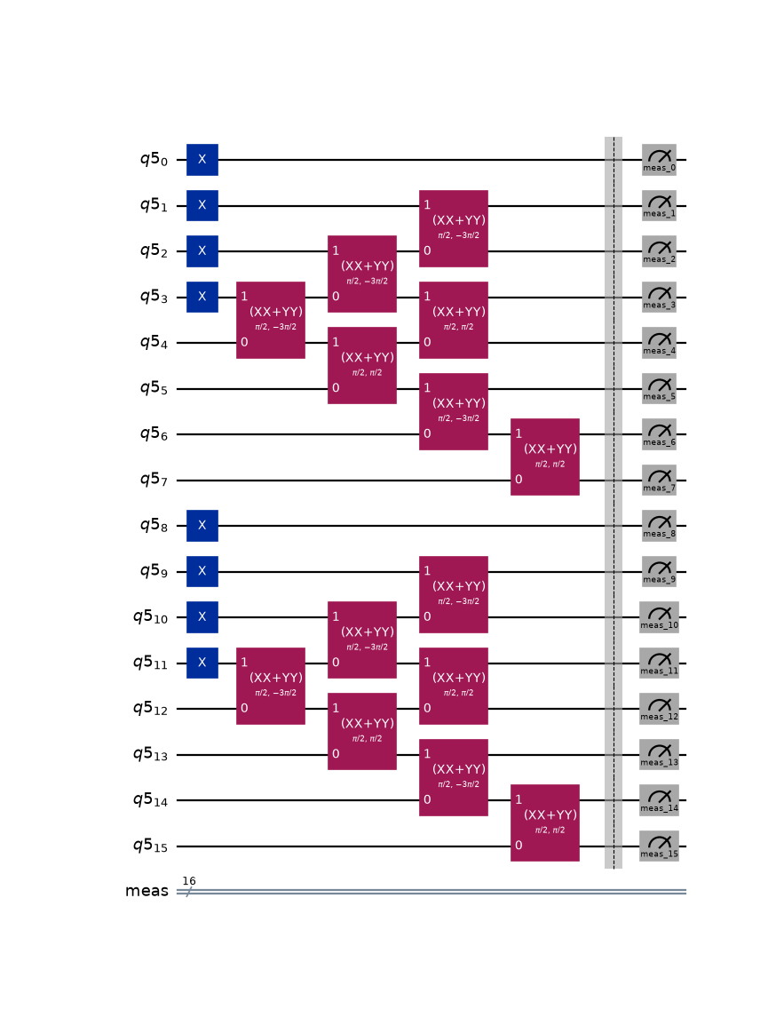
The Krylov dimension shows up directly in the circuits’ two-qubit depth: the reference-state preparation is a fixed cost, and each additional Krylov power adds another second-order Trotter step of the time-evolution operator.

>>> two_qubit = lambda instr: instr.operation.num_qubits == 2
>>> [circuit.depth(two_qubit) for circuit in circuits]
[4, 12, 21, 30, 39]

Note

Splitting the Hamiltonian is what keeps these depths modest. The one-body evolution is a genuine orbital rotation, so it synthesizes to an XXPlusYYGate brickwork on adjacent qubits, while each half-step of the on-site interaction is a single RZZGate coupling the impurity’s two spin modes – the cheap term the second-order product sandwiches around the rotation. Handing the whole Hamiltonian to one Evolution gate instead would Pauli-Trotterize the one-body part term by term, dragging long Jordan-Wigner Z-strings through the (long-range) impurity–bath couplings and inflating the depth by an order of magnitude.

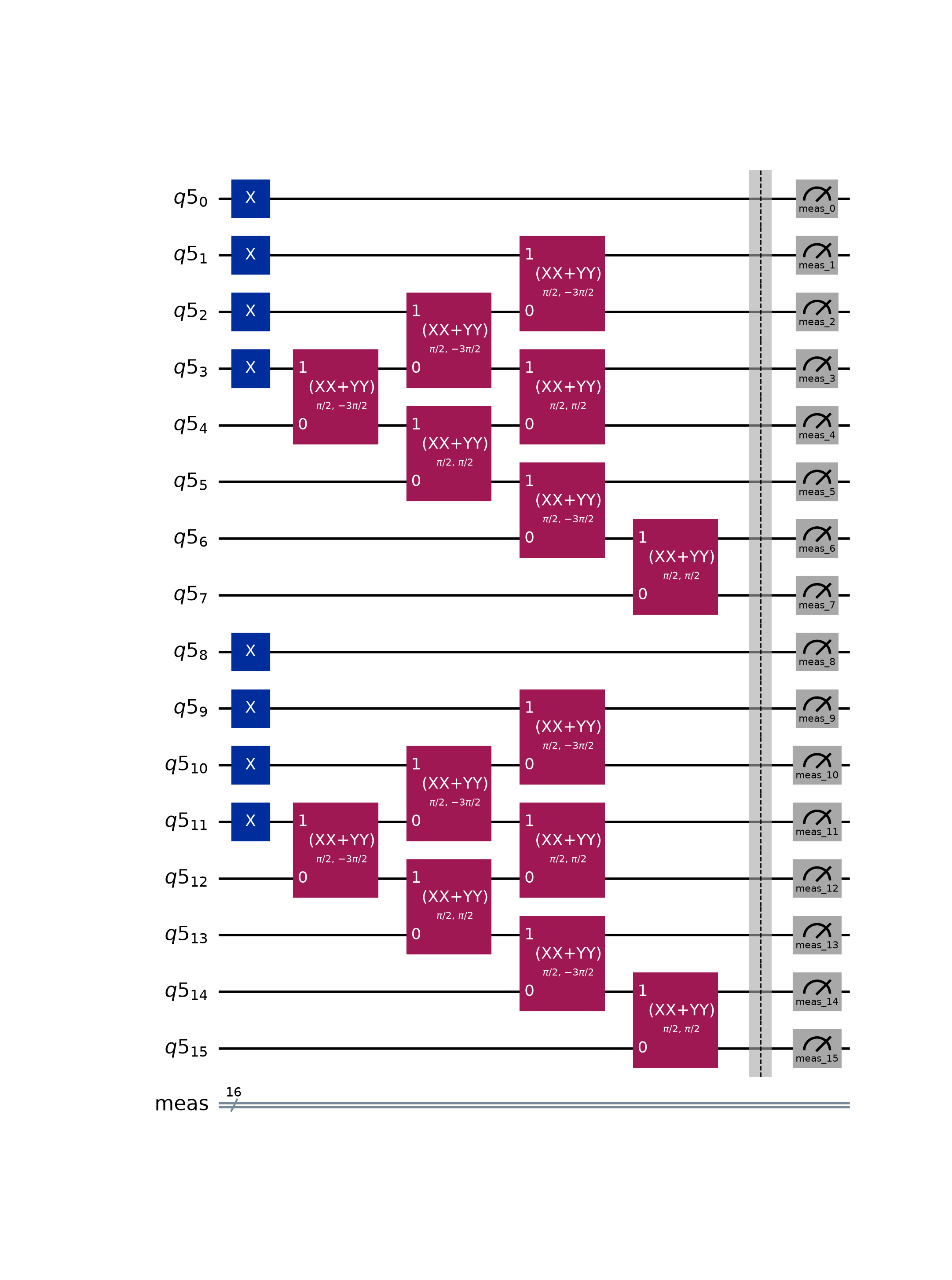
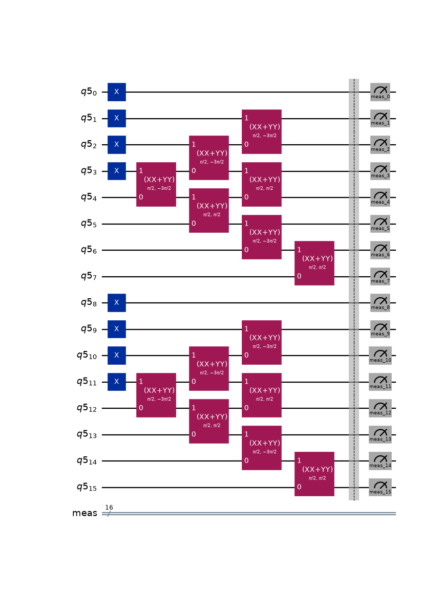
The first circuit prepares only the reference determinant, while the last carries the most Trotter steps (4 in this case):

>>> circuits[0].draw("mpl", fold=-1, measure_arrows=False)
<Figure size ... with 1 Axes>

(png, hires.png, pdf)

>>> circuits[-1].draw("mpl", fold=-1, measure_arrows=False)
<Figure size ... with 1 Axes>

(png, hires.png, pdf)

6. Sample bitstrings from the Krylov circuits

On hardware, we would run the transpiled circuits and measure. Here we do the noiseless (statevector) version of that step to see the bitstrings SKQD would collect. We simulate each untranspiled FermionicCircuit with ffsim.apply_unitary() and sample the resulting statevector with ffsim.sample_state_vector().

Because a PrepareSlaterDeterminant gate is validate-then-rotate under simulation (it checks that the incoming state occupies its reference determinant, then applies the rotation), the input is the plain occupation determinant – the lowest nocc modes filled per spin, with no rotation. The gate applies reference_rotation itself.

>>> import ffsim
>>> from collections import Counter
>>>
>>> reference = ffsim.slater_determinant(
...     norb, (list(range(nelec[0])), list(range(nelec[1])))
... )
>>>
>>> shots = 1000
>>> counts = Counter()
>>> for dim, fermionic_circuit in enumerate(fermionic_circuits):
...     statevector = ffsim.apply_unitary(reference, fermionic_circuit, norb=norb, nelec=nelec)
...     samples = ffsim.sample_state_vector(
...         statevector, norb=norb, nelec=nelec, shots=shots, seed=dim
...     )
...     counts += Counter(samples)

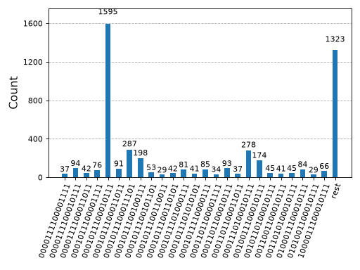
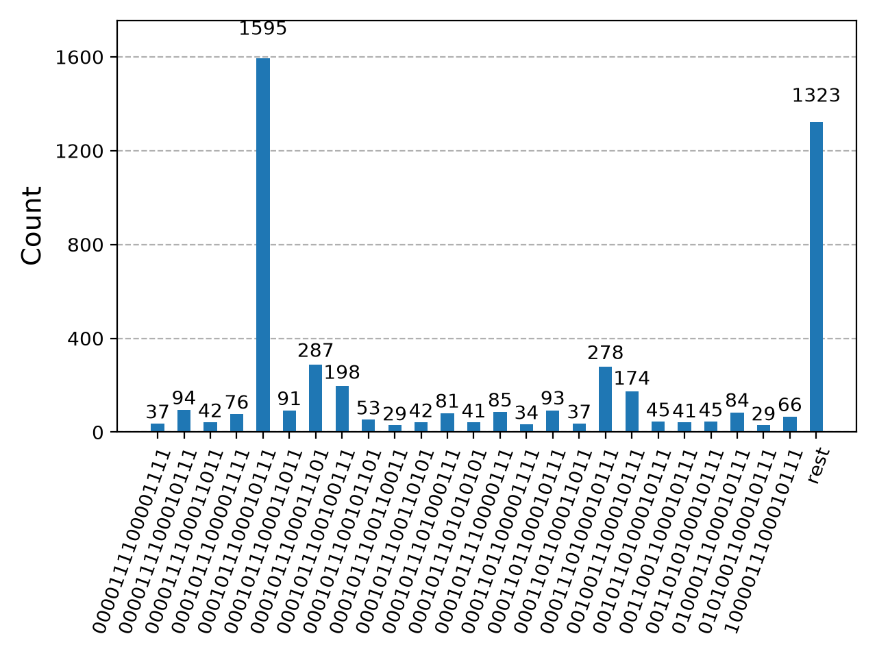
Pooling the samples from all five Krylov circuits, the support is tiny: a few hundred distinct bitstrings out of the \(\binom{8}{4}^2 = 4900\) determinants in the (4, 4) sector. This concentration – a direct consequence of the momentum-basis sparsity established in step 2 – is exactly what makes the subsequent classical diagonalization tractable.

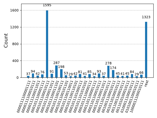
Plotting the counts with qiskit.visualization.plot_histogram() makes the sparsity visible – a handful of configurations dominate, led by the reference determinant.

>>> from qiskit.visualization import plot_histogram
>>>
>>> plot_histogram(dict(counts), number_to_keep=25)
<Figure size ... with 1 Axes>

(png, hires.png, pdf)

7. Diagonalize in the sampled subspace

The sampled bitstrings are the input to the classical half of SKQD: the Hamiltonian is projected onto the subspace the sampled configurations span and diagonalized there. We hand this off to the qiskit-addon-sqd package, whose diagonalize_fermionic_hamiltonian() runs the full sample-based quantum diagonalization loop: it builds a subspace from batches of the sampled configurations, diagonalizes the Hamiltonian in it, and iteratively refines the subspace via configuration recovery – flipping occupations to repair configurations that violate the known particle-number symmetry. Configuration recovery is designed to undo the damage of hardware noise, which corrupts sampled bitstrings into the wrong particle-number sector; we sample noiselessly here, so there is nothing to repair on that front.

The solver consumes the sampled counts as a BitArray, which we build directly from the pooled counts of step 6. It diagonalizes in the same momentum basis the rest of the construction uses, so it takes the h1e_momentum and h2e_momentum integrals from step 2 directly – no repacking. The recovered energy matches the exact reference to well under a milli-Hartree, from only a few hundred sampled configurations; because the SQD energy is a variational upper bound on the true ground state, it always sits at or above reference_energy (still in scope from step 2):

>>> from qiskit.primitives import BitArray
>>> from qiskit_addon_sqd.fermion import diagonalize_fermionic_hamiltonian
>>>
>>> bit_array = BitArray.from_counts(dict(counts))
>>>
>>> # record each iteration's batch results so we can watch the energy converge
>>> result_history = []
>>> result = diagonalize_fermionic_hamiltonian(
...     h1e_momentum,
...     h2e_momentum,
...     bit_array,
...     samples_per_batch=100,
...     norb=norb,
...     nelec=nelec,
...     num_batches=3,
...     max_iterations=3,
...     symmetrize_spin=True,
...     callback=result_history.append,
...     seed=np.random.default_rng(24),
... )
>>> print(f"SQD estimate: {result.energy:.4f} (exact: {reference_energy:.4f})")
SQD estimate: -13.4224 (exact: -13.4225)

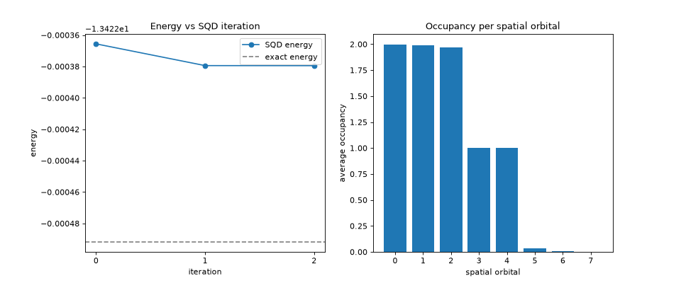
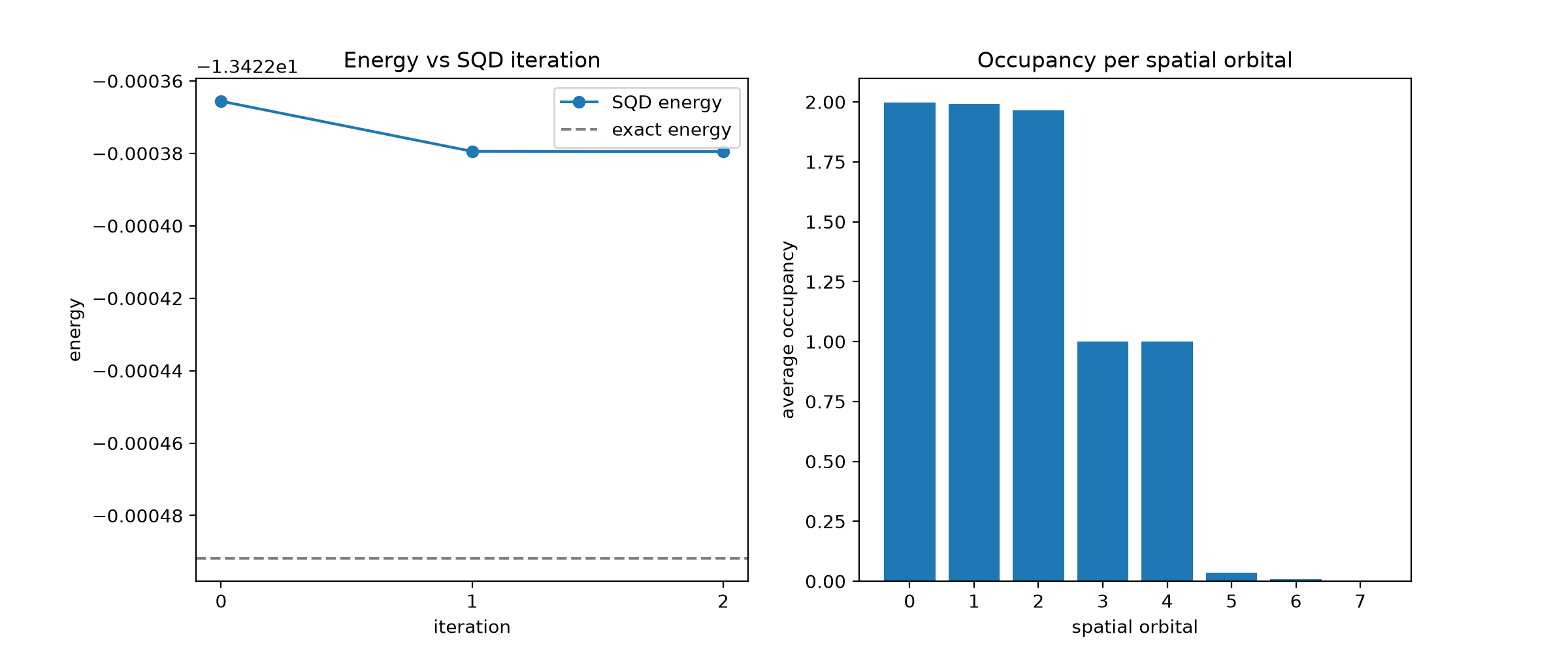
Finally, we visualize the run: the energy’s convergence across the iterations, and the average occupancy of each spatial orbital in the recovered ground state. The per-iteration energy is the lowest across that iteration’s batches, and the occupancy sums the orbital_occupancies over the two spin sectors. Even without noise to correct, the energy still decreases from iteration to iteration: each iteration diagonalizes within num_batches batches of only samples_per_batch configurations subsampled from the pool, and the iterative refinement due to bitstring carryover steadily improves which configurations land in those batches – so the recovered energy improves:

>>> import matplotlib.pyplot as plt
>>> from matplotlib.ticker import MaxNLocator
>>>
>>> min_energies = [min(batch, key=lambda r: r.energy).energy for batch in result_history]
>>> occupancies = np.sum(result.orbital_occupancies, axis=0)
>>>
>>> fig, axs = plt.subplots(1, 2, figsize=(12, 5))
>>> _ = axs[0].plot(range(len(min_energies)), min_energies, marker="o", label="SQD energy")
>>> _ = axs[0].axhline(reference_energy, color="gray", linestyle="--", label="exact energy")
>>> _ = axs[0].set_xlabel("iteration")
>>> _ = axs[0].set_ylabel("energy")
>>> _ = axs[0].set_title("Energy vs SQD iteration")
>>> _ = axs[0].xaxis.set_major_locator(MaxNLocator(integer=True))
>>> _ = axs[0].legend()
>>> _ = axs[1].bar(range(norb), occupancies)
>>> _ = axs[1].set_xlabel("spatial orbital")
>>> _ = axs[1].set_ylabel("average occupancy")
>>> _ = axs[1].set_title("Occupancy per spatial orbital")
>>> fig
<Figure size ... with 2 Axes>

(png, hires.png, pdf)

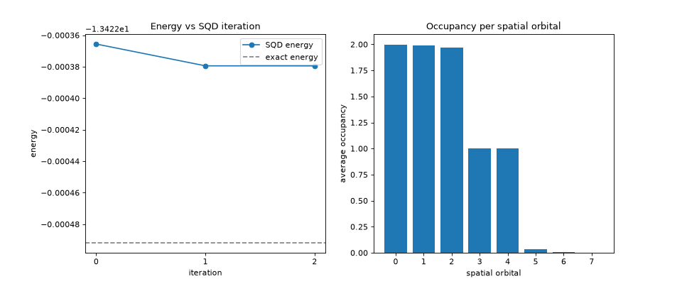
This closes the SKQD loop: the momentum-basis circuits of steps 1–5 produce a sparse sample (step 6), and the sample-based diagonalization above turns that sample back into a ground-state energy.

Next steps

This guide ran the whole SKQD pipeline on a noiseless statevector simulator. On hardware, the transpiled circuits would be executed and measured in place of the statevector sampling of step 6, with the resulting counts feeding the same step-7 diagonalization unchanged. Refer to the Qiskit documentation for running circuits, and to the SQD addon tutorials for more on the subspace-diagonalization post-processing – including its behavior on noisy samples, where configuration recovery does the most work.

Read the ffsim backend guide to understand why ffsim.apply_unitary() and ffsim.sample_state_vector() work natively on this package’s fermionic circuits, and why the fixed-particle-number sector used in step 6 is what makes the momentum-basis sparsity established in step 2 sample-efficient in the first place.