Build an LUCJ ansatz
Important
The concepts in this guide are currently available only in the Python API. Equivalent functionality will be made available through the C API in a future release.
The local unitary cluster Jastrow (LUCJ) ansatz is a compact, hardware-efficient parametrization of a correlated electronic wavefunction. It is a member of the more general unitary cluster Jastrow (UCJ) family and takes the form
where \(\lvert \Phi_0 \rangle\) is a reference state (typically Hartree-Fock), each \(\mathcal{U}_k\) is an orbital rotation, and each \(\mathcal{J}_k\) is a diagonal Coulomb operator
with \(n_{i\sigma}\) the number operator on spatial orbital \(i\) with spin
\(\sigma\). This guide shows how to assemble such an ansatz for a real molecule using the
UCJ gate from qiskit_fermions.circuit.library.
1. Run the classical calculation
The (L)UCJ ansatz can be initialized from the amplitudes of a coupled-cluster singles and
doubles (CCSD) calculation. Here we run restricted Hartree-Fock followed by CCSD for a hydrogen
molecule in the 6-31g basis, using PySCF for the quantum chemistry.
>>> import pyscf
>>> import pyscf.cc
>>>
>>> # build the molecule and run Hartree-Fock
>>> mol = pyscf.gto.Mole()
>>> mol.build(
...     atom=[["H", (0, 0, 0)], ["H", (0, 0, 0.74)]],
...     basis="6-31g",
...     symmetry="Dooh",
...     verbose=0,
... )
<pyscf.gto.mole.Mole object at ...>
>>> scf = pyscf.scf.RHF(mol).run()
>>>
>>> mo_coeff = scf.mo_coeff
>>> norb = mo_coeff.shape[1]
>>> nelec = (mol.nelec[0], mol.nelec[1])
>>>
>>> # run CCSD for the t-amplitudes
>>> ccsd = pyscf.cc.CCSD(scf).run()
>>> t1, t2 = ccsd.t1, ccsd.t2
2. Build the molecular Hamiltonian as a fermionic operator
We will need the Hamiltonian later to evaluate the ansatz energy. We build it directly as a
FermionOperator from the molecular-orbital integrals: the one-body integrals h1e
(the core Hamiltonian in the MO basis), the two-body integrals h2e (from pyscf.ao2mo()),
and the constant nuclear-repulsion energy. The electronic-integral constructors
from_1body_tril_spin_sym() and
from_2body_tril_spin_sym() expect the integrals
in packed (lower-triangular) chemist ordering, which is exactly what PySCF produces.
>>> from pyscf import ao2mo, lib
>>>
>>> from qiskit_fermions.operators import FermionOperator
>>>
>>> # one- and two-body molecular-orbital integrals and the nuclear-repulsion energy
>>> h1e = mo_coeff.T @ scf.get_hcore() @ mo_coeff
>>> h2e = ao2mo.kernel(mol, mo_coeff)
>>> ecore = mol.energy_nuc()
>>>
>>> # pack into the lower-triangular chemist-ordered layout the constructors expect
>>> h1e_tril = lib.pack_tril(h1e)
>>> h2e_tril = lib.pack_tril(h2e)
>>>
>>> hamiltonian = ecore * FermionOperator.one()
>>> hamiltonian += FermionOperator.from_1body_tril_spin_sym(h1e_tril, norb)
>>> hamiltonian += FermionOperator.from_2body_tril_spin_sym(h2e_tril, norb)
3. Build the LUCJ circuit
The UCJ gate assembles the ansatz directly from the coupled-cluster amplitudes. Its
from_t_amplitudes() constructor performs a double
factorization of the \(t_2\) amplitudes (via
double_factorized_t2()) to obtain the per-layer diagonal Coulomb
matrices and orbital rotations, and derives an optional final orbital rotation from the
\(t_1\) amplitudes.
The number of ansatz repetitions \(L\) equals the number of terms in the double
factorization. Truncating it with the n_reps argument trades some accuracy for a shallower
circuit; here we keep the two largest terms, which recovers most of the correlation energy while
halving the number of layers.
>>> from qiskit_fermions.circuit import FermionicCircuit
>>> from qiskit_fermions.circuit.library import InitializeModes, UCJ
>>>
>>> ansatz = UCJ.from_t_amplitudes(nelec, t2, t1=t1, n_reps=2)
>>>
>>> circuit = FermionicCircuit(2 * norb)
>>> circuit.append(InitializeModes.from_hartree_fock(norb, nelec), circuit.modes)
>>> circuit.append(ansatz, circuit.modes)
The UCJ gate is a pure unitary carrying no reference of its own, so we prepend an
InitializeModes gate (built with
from_hartree_fock()) to supply the
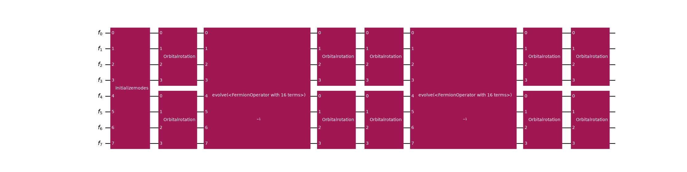
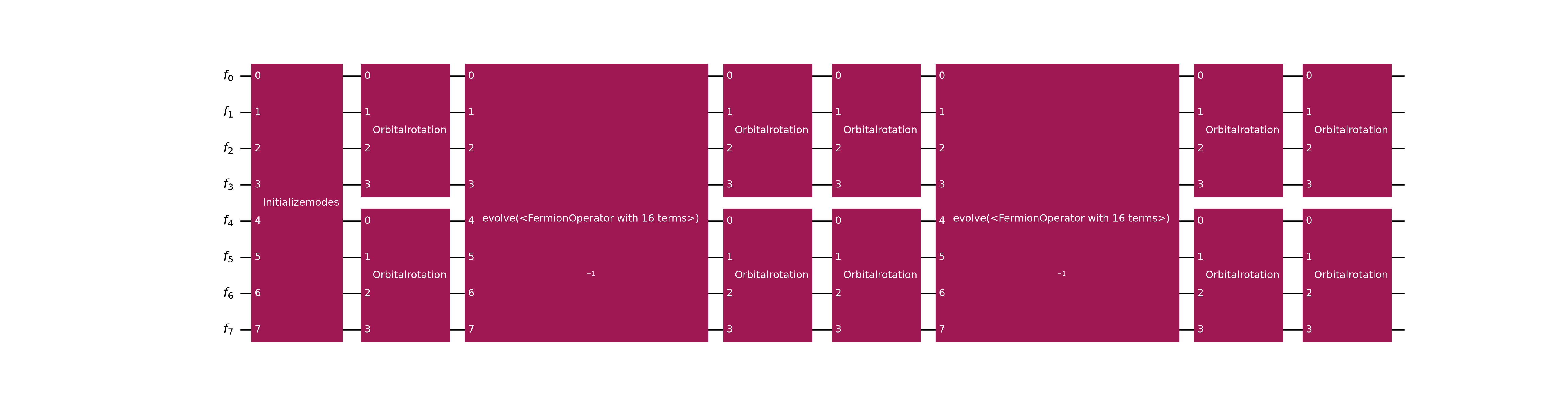
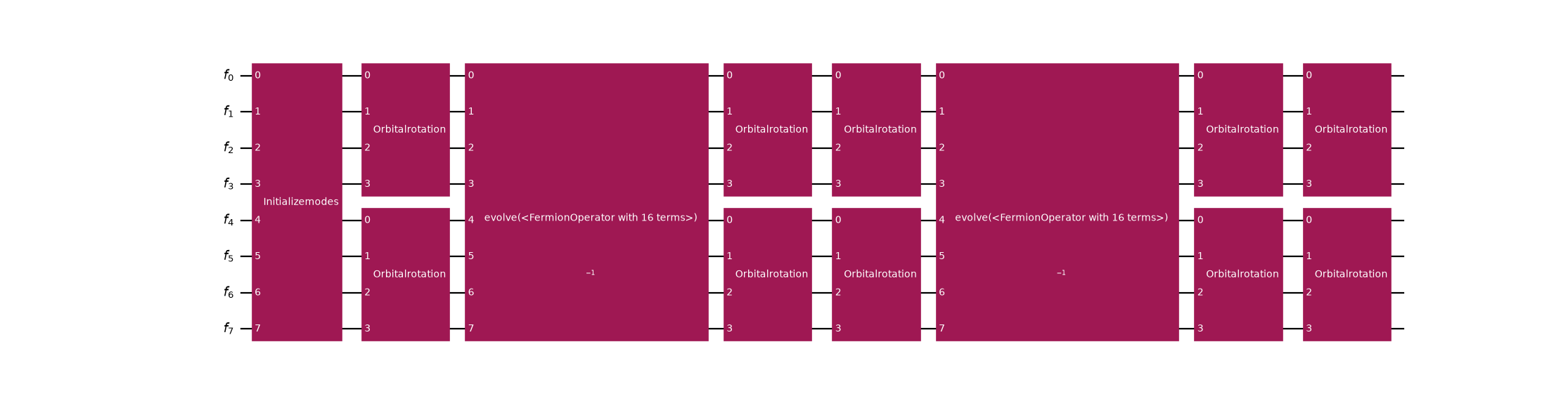
Hartree-Fock reference the ansatz is applied to. Decomposing the circuit reveals its anatomy: the
InitializeModes gate prepares the reference determinant, and each ansatz layer contributes
an OrbitalRotation \(\mathcal{U}_k^\dagger\), then \(e^{i\mathcal{J}_k}\) (an
Evolution of the diagonal Coulomb operator \(\mathcal{J}_k\)), then
\(\mathcal{U}_k\), with a final OrbitalRotation at the end. The orbital rotations act
per spin sector, so each is placed on the alpha modes 0..norb and the beta modes
norb..2*norb independently.
>>> circuit.decompose().draw("mpl", fold=-1)
<Figure size ... with 1 Axes>
Note
Each layer ends with \(\mathcal{U}_k\) and the next begins with
\(\mathcal{U}_{k+1}^\dagger\), so adjacent OrbitalRotation gates could be merged
into a single rotation. A transpilation pass performing this fusion is a planned future
development.
4. Simulate the ansatz and evaluate its energy
Because every gate in the circuit implements ffsim’s ffsim.SupportsApplyUnitary protocol,
the whole FermionicCircuit can be applied to a fixed particle-number state vector with
ffsim.apply_unitary(), starting from the Hartree-Fock reference. The
FermionOperator likewise implements ffsim’s ffsim.SupportsLinearOperator
protocol, so we can obtain a SciPy LinearOperator for it via
ffsim.linear_operator() and evaluate the ansatz energy as the expectation value of the
molecular Hamiltonian.
>>> import ffsim
>>> import numpy as np
>>>
>>> reference = ffsim.hartree_fock_state(norb, nelec)
>>> state = ffsim.apply_unitary(reference, circuit, norb=norb, nelec=nelec)
>>>
>>> linop = ffsim.linear_operator(hamiltonian, norb=norb, nelec=nelec)
>>> energy = np.vdot(state, linop @ state).real
>>> print(f"LUCJ energy: {energy:.8f} Hartree")
LUCJ energy: -1.14618323 Hartree
The LUCJ energy improves substantially on the Hartree-Fock reference and approaches the CCSD energy it was initialized from – the small remaining gap is the price of truncating the ansatz to two repetitions:
>>> print(f"Hartree-Fock: {scf.e_tot:.8f} Hartree")
Hartree-Fock: -1.12675532 Hartree
>>> print(f"CCSD:         {ccsd.e_tot:.8f} Hartree")
CCSD:         -1.15167268 Hartree
5. (Optional) Use ffsim’s compressed double factorization
The UCJ gate above is initialized from an exact double factorization of the \(t_2\)
amplitudes: the number of ansatz repetitions \(L\) is whatever that factorization yields (up to
the n_reps truncation), and each layer reproduces one factorized term exactly. ffsim
additionally offers an optimized (“compressed”) double factorization – its
from_t_amplitudes(..., optimize=True) – which variationally fits the amplitudes with a chosen,
typically smaller, number of repetitions. This trades a classical optimization up front for a
shallower ansatz at a target accuracy, and has no equivalent in this package.
There is no need to re-implement it: an ffsim UCJ operator exposes the same tensors that
UCJ is built from, so we can construct the operator with optimize=True and hand its
diag_coulomb_mats / orbital_rotations / final_orbital_rotation straight to the
UCJ constructor.
>>> compressed = ffsim.UCJOpSpinBalanced.from_t_amplitudes(
...     t2, t1=t1, n_reps=2, optimize=True
... )
>>>
>>> compressed_ansatz = UCJ(
...     "balanced",
...     compressed.diag_coulomb_mats,
...     compressed.orbital_rotations,
...     final_orbital_rotation=compressed.final_orbital_rotation,
... )
>>>
>>> compressed_circuit = FermionicCircuit(2 * norb)
>>> compressed_circuit.append(
...     InitializeModes.from_hartree_fock(norb, nelec), compressed_circuit.modes
... )
>>> compressed_circuit.append(compressed_ansatz, compressed_circuit.modes)
The resulting circuit is used exactly like the one built from the exact factorization – the
UCJ gate does not care how its tensors were obtained – and evaluating its energy the same
way recovers the same correlation energy at this (small) system size:
>>> state = ffsim.apply_unitary(reference, compressed_circuit, norb=norb, nelec=nelec)
>>> energy = np.vdot(state, linop @ state).real
>>> print(f"compressed LUCJ energy: {energy:.8f} Hartree")
compressed LUCJ energy: -1.14618323 Hartree
Note
diag_coulomb_mats from optimize=True may carry tiny imaginary round-off; UCJ
takes their real part and raises only if the imaginary part is not negligible. For a better fit at
a given n_reps (at increased classical cost) see ffsim’s multi_stage_start /
multi_stage_step options.
6. Transpile the ansatz to a qubit circuit
To run the ansatz on hardware it must be lowered from fermionic modes to qubits.
The generate_preset_jw_pass_manager() preset builds a
staged pipeline that maps the fermionic circuit through the Jordan-Wigner transformation and
synthesizes each gate into a qubit-level circuit. The composite UCJ gate must first be
decomposed into its primitive gates (OrbitalRotation, Evolution, …) so the
pipeline’s optimization stage can act on them – so we pass circuit.decompose().
>>> from qiskit_fermions.transpiler.presets import generate_preset_jw_pass_manager
>>>
>>> # ``circuit`` is the exact-factorization ansatz assembled in step 3
>>> pm = generate_preset_jw_pass_manager()
>>> transpiled = pm.run(circuit.decompose())
>>> print(dict(sorted(transpiled.count_ops().items())))
{'p': 16, 'rzz': 12, 'x': 2, 'xx_plus_yy': 28}
Without a target device this maps onto 2 * norb qubits with all-to-all connectivity assumed; the
orbital rotations synthesize into XXPlusYYGates and the diagonal
Coulomb evolutions into RZZGates:
>>> transpiled.draw("mpl", fold=-1)
<Figure size ... with 1 Axes>



Targeting hardware connectivity with ffsim’s LUCJ pass manager
A real device has a restricted qubit coupling map, and the LUCJ ansatz is designed to match it: the
same-spin (pairs_aa) interactions form two linear chains and the alpha-beta (pairs_ab)
interactions bridge them. ffsim’s generate_lucj_pass_manager() builds a
device-aware qubit pipeline for exactly this structure – and returns the subset of pairs_ab the
hardware can actually accommodate. We can slot that pipeline into the preset’s qubit stage while
keeping our own fermion-to-qubit synthesis:
>>> from ffsim.qiskit import generate_lucj_pass_manager
>>> from qiskit.providers.fake_provider import GenericBackendV2
>>> from qiskit.transpiler import CouplingMap
>>>
>>> # a heavy-hex device coupling map (any BackendV2 works, e.g. a real fake_provider backend)
>>> coupling_map = CouplingMap.from_heavy_hex(5)
>>> backend = GenericBackendV2(
...     num_qubits=coupling_map.size(),
...     basis_gates=["cp", "xx_plus_yy", "p", "x", "swap"],
...     coupling_map=coupling_map,
... )
>>>
>>> # nearest-neighbor same-spin chain; let the pass manager choose the alpha-beta pairs
>>> pairs_aa = [(p, p + 1) for p in range(norb - 1)]
>>>
>>> pm = generate_preset_jw_pass_manager()
>>> pm.qubit, allowed_pairs_ab = generate_lucj_pass_manager(
...     backend, norb, "heavy-hex", (pairs_aa, None), optimization_level=3, seed_transpiler=0
... )
>>>
>>> # the alpha-beta interactions the heavy-hex connectivity can implement
>>> print(allowed_pairs_ab)
[(0, 0)]
With pm.qubit now set to the device-aware pipeline, running the pass manager lays the circuit out
on the backend’s qubits and routes it to the coupling map. If we route the unrestricted ansatz from
step 3 – whose diagonal Coulomb operator still contains alpha-beta terms the hardware cannot reach
directly – the router must insert many SWAP gates to bridge them:
>>> naive = pm.run(circuit.decompose())
>>> naive.num_qubits  # laid out on the full heavy-hex device register
57
>>> naive_swaps = naive.count_ops()["swap"]
>>> naive_swaps  # many SWAPs to bridge the unreachable alpha-beta interactions
33
Restricting the ansatz to the hardware-implementable interactions
The fix is to feed allowed_pairs_ab back into the ansatz construction – via the
interaction_pairs argument of from_t_amplitudes() –
so the diagonal Coulomb operator only contains alpha-beta terms the coupling map can implement
directly. The ansatz then matches the device topology and the router barely has to touch it:
>>> restricted = UCJ.from_t_amplitudes(
...     nelec, t2, t1=t1, n_reps=2, interaction_pairs=(pairs_aa, allowed_pairs_ab)
... )
>>>
>>> circuit = FermionicCircuit(2 * norb)
>>> circuit.append(InitializeModes.from_hartree_fock(norb, nelec), circuit.modes)
>>> circuit.append(restricted, circuit.modes)
>>>
>>> transpiled = pm.run(circuit.decompose())
>>> restricted_swaps = transpiled.count_ops()["swap"]
>>> restricted_swaps  # far fewer routing SWAPs than the unrestricted ansatz
4
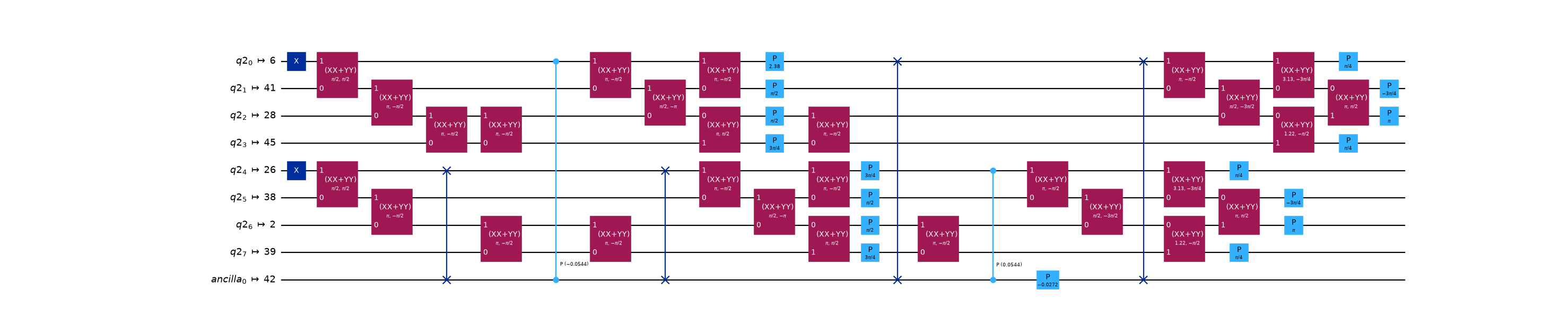
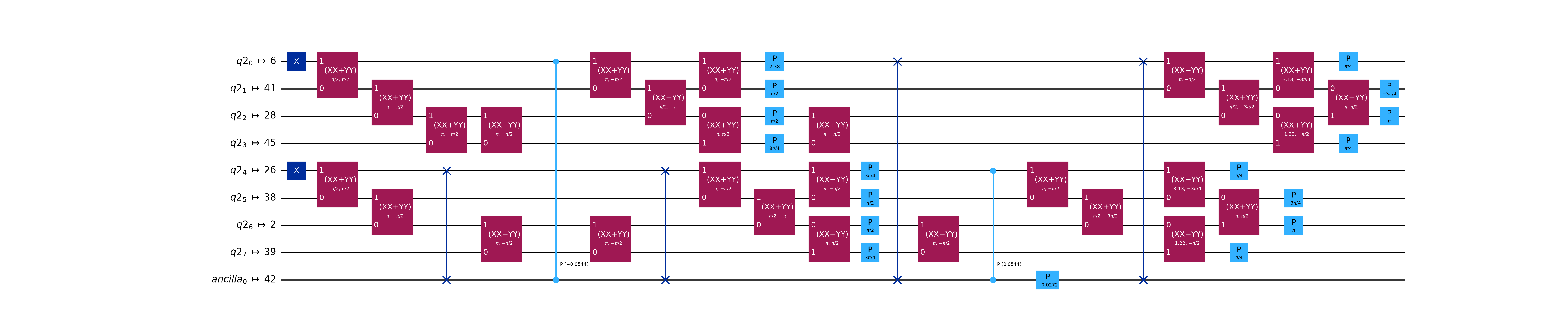
Drawing only the active qubits (idle_wires=False) shows the circuit restricted to the two spin
chains and the alpha-beta bridge, expressed in the device basis gates. Layout and routing scatter the
logical modes across the device’s physical qubits, so we pass a wire_order taken from the
circuit’s final layout – final_index_layout() lists the
physical qubit each input qubit ended up on, in input-qubit order – to draw the wires back in the
original mode order:
>>> wire_order = transpiled.layout.final_index_layout(filter_ancillas=False)
>>> transpiled.draw("mpl", idle_wires=False, fold=-1, wire_order=wire_order)
<Figure size ... with 1 Axes>
Note
The exact post-layout gate counts and depth depend on the routing/optimization passes and the
chosen device, so they are not reproduced here. The key point is the co-design: expressing the
ansatz with a nearest-neighbor pairs_aa chain and hardware-filtered pairs_ab bridges keeps
the synthesized circuit close to the device topology, minimizing the routing overhead (inserted
SWAP gates). See GivensDecompositionSlaterDeterminantSynthesis for a related
synthesis choice (minimize_2q_gate_count) trading two-qubit gate count against routed depth.
Next steps
Learn how the individual gates work in the
qiskit_fermions.circuit.librarydocumentation and the fermionic circuit guide.Explore the operators explanation guide to understand how to construct fermionic Hamiltonians such as the diagonal Coulomb operator used above.
See how a fermionic circuit is mapped to qubits in the transpilation guide.
Read the ffsim backend guide to understand why
ffsim.apply_unitary()andffsim.linear_operator()work natively on this ansatz, and how to evaluate its energy without ffsim installed.