Minimum eigenvalue estimation of a spin (qubit) Hamiltonian
In this tutorial we implement a Qiskit pattern showing how to post-process quantum samples to approximate the minimum eigenvalue and spin-spin correlators for a 22-site XX-Z spin-1/2 chain. We will follow a sample-based quantum diagonalization approach [1].
While a Qiskit pattern typically involves 4 steps, the aim of this tutorial is to focus on the post-processing of the samples obtained from a quantum circuit whose support coincides with that of the eigenstate corresponding to the minimum eigenvalue. Consequently, we generate a synthetic set of bitstrings to define the subspace and do not design an ansatz nor sample from a quantum circuit in this tutorial.
The pattern we will implement is as follows:
Step 1: Map to quantum problem
Specify a Hamiltonian as a Pauli operator
Step 2: Optimize the problem
N/A
Step 3: Execute experiments
N/A: Will generate synthetic quantum samples
Step 4: Post-process results
Project the Hamiltonian onto the subspace spanned by the samples
Diagonalize the Hamiltonian in the subspace to approximate the minimum eigenstate
Calculate spin-spin correlators for each site, \(l\)
Step 1: Map to quantum problem
The Hamiltonian of interest can be written as:
with \(\alpha_i\) being real coefficients and \(P_i\) Pauli strings. A wide class of many-body Hamiltonians can be written as the linear combination of polynomially-many Pauli strings, including interacting-electron Hamiltonians, spin Hamiltonians, etc.
In particular, we consider the properties of the antiferromagnetic XX-Z spin-1/2 chain with \(L = 22\) sites:
[1]:
from qiskit.transpiler import CouplingMap
from qiskit_addon_utils.problem_generators import generate_xyz_hamiltonian

num_spins = 22
coupling_map = CouplingMap.from_ring(num_spins)
hamiltonian = generate_xyz_hamiltonian(coupling_map, coupling_constants=(0.3, 0.3, 1.0))
print(hamiltonian)
SparsePauliOp(['IIIIIIIIIIIIIIIIIIIIXX', 'IIIIIIIIIIIIIIIIIIIIYY', 'IIIIIIIIIIIIIIIIIIIIZZ', 'IIIIIIIIIIIIIIIIIIXXII', 'IIIIIIIIIIIIIIIIIIYYII', 'IIIIIIIIIIIIIIIIIIZZII', 'IIIIIIIIIIIIIIIIXXIIII', 'IIIIIIIIIIIIIIIIYYIIII', 'IIIIIIIIIIIIIIIIZZIIII', 'IIIIIIIIIIIIIIXXIIIIII', 'IIIIIIIIIIIIIIYYIIIIII', 'IIIIIIIIIIIIIIZZIIIIII', 'IIIIIIIIIIIIXXIIIIIIII', 'IIIIIIIIIIIIYYIIIIIIII', 'IIIIIIIIIIIIZZIIIIIIII', 'IIIIIIIIIIXXIIIIIIIIII', 'IIIIIIIIIIYYIIIIIIIIII', 'IIIIIIIIIIZZIIIIIIIIII', 'IIIIIIIIXXIIIIIIIIIIII', 'IIIIIIIIYYIIIIIIIIIIII', 'IIIIIIIIZZIIIIIIIIIIII', 'IIIIIIXXIIIIIIIIIIIIII', 'IIIIIIYYIIIIIIIIIIIIII', 'IIIIIIZZIIIIIIIIIIIIII', 'IIIIXXIIIIIIIIIIIIIIII', 'IIIIYYIIIIIIIIIIIIIIII', 'IIIIZZIIIIIIIIIIIIIIII', 'IIXXIIIIIIIIIIIIIIIIII', 'IIYYIIIIIIIIIIIIIIIIII', 'IIZZIIIIIIIIIIIIIIIIII', 'XXIIIIIIIIIIIIIIIIIIII', 'YYIIIIIIIIIIIIIIIIIIII', 'ZZIIIIIIIIIIIIIIIIIIII', 'XIIIIIIIIIIIIIIIIIIIIX', 'YIIIIIIIIIIIIIIIIIIIIY', 'ZIIIIIIIIIIIIIIIIIIIIZ', 'IIIIIIIIIIIIIIIIIIIXXI', 'IIIIIIIIIIIIIIIIIIIYYI', 'IIIIIIIIIIIIIIIIIIIZZI', 'IIIIIIIIIIIIIIIIIXXIII', 'IIIIIIIIIIIIIIIIIYYIII', 'IIIIIIIIIIIIIIIIIZZIII', 'IIIIIIIIIIIIIIIXXIIIII', 'IIIIIIIIIIIIIIIYYIIIII', 'IIIIIIIIIIIIIIIZZIIIII', 'IIIIIIIIIIIIIXXIIIIIII', 'IIIIIIIIIIIIIYYIIIIIII', 'IIIIIIIIIIIIIZZIIIIIII', 'IIIIIIIIIIIXXIIIIIIIII', 'IIIIIIIIIIIYYIIIIIIIII', 'IIIIIIIIIIIZZIIIIIIIII', 'IIIIIIIIIXXIIIIIIIIIII', 'IIIIIIIIIYYIIIIIIIIIII', 'IIIIIIIIIZZIIIIIIIIIII', 'IIIIIIIXXIIIIIIIIIIIII', 'IIIIIIIYYIIIIIIIIIIIII', 'IIIIIIIZZIIIIIIIIIIIII', 'IIIIIXXIIIIIIIIIIIIIII', 'IIIIIYYIIIIIIIIIIIIIII', 'IIIIIZZIIIIIIIIIIIIIII', 'IIIXXIIIIIIIIIIIIIIIII', 'IIIYYIIIIIIIIIIIIIIIII', 'IIIZZIIIIIIIIIIIIIIIII', 'IXXIIIIIIIIIIIIIIIIIII', 'IYYIIIIIIIIIIIIIIIIIII', 'IZZIIIIIIIIIIIIIIIIIII'],
              coeffs=[0.3+0.j, 0.3+0.j, 1. +0.j, 0.3+0.j, 0.3+0.j, 1. +0.j, 0.3+0.j, 0.3+0.j,
 1. +0.j, 0.3+0.j, 0.3+0.j, 1. +0.j, 0.3+0.j, 0.3+0.j, 1. +0.j, 0.3+0.j,
 0.3+0.j, 1. +0.j, 0.3+0.j, 0.3+0.j, 1. +0.j, 0.3+0.j, 0.3+0.j, 1. +0.j,
 0.3+0.j, 0.3+0.j, 1. +0.j, 0.3+0.j, 0.3+0.j, 1. +0.j, 0.3+0.j, 0.3+0.j,
 1. +0.j, 0.3+0.j, 0.3+0.j, 1. +0.j, 0.3+0.j, 0.3+0.j, 1. +0.j, 0.3+0.j,
 0.3+0.j, 1. +0.j, 0.3+0.j, 0.3+0.j, 1. +0.j, 0.3+0.j, 0.3+0.j, 1. +0.j,
 0.3+0.j, 0.3+0.j, 1. +0.j, 0.3+0.j, 0.3+0.j, 1. +0.j, 0.3+0.j, 0.3+0.j,
 1. +0.j, 0.3+0.j, 0.3+0.j, 1. +0.j, 0.3+0.j, 0.3+0.j, 1. +0.j, 0.3+0.j,
 0.3+0.j, 1. +0.j])
Step 2: Optimize problem (N/A)
This tutorial is focused on post-processing samples taken from a QPU. Discussion on generating an ansatz and optimizing it for QPU execution is out of scope.
Step 3: Execute experiments
This tutorial is focused on post-processing samples taken from a QPU. Discussion on running a specific state-preparation ansatz for a given Hamiltonian is out of scope. Since we don’t have a specific circuit for which to evaluate the Hamiltonian, we will generate a set of synthetic samples which cover all possible pairs of domain walls.
[2]:
import numpy as np

bitstring_matrix = np.array([[i % 2 == 0 for i in range(num_spins)]], dtype=bool)
bitstring_matrix = np.concatenate((bitstring_matrix, np.roll(bitstring_matrix, 1, axis=1)))
for i in range(num_spins):
    for j in range(num_spins // 2):
        domain_wall = bitstring_matrix[0].copy()
        domain_wall[i] -= 1
        domain_wall[(i + 1 + j * 2) % num_spins] -= 1
        bitstring_matrix = np.concatenate((bitstring_matrix, np.expand_dims(domain_wall, axis=0)))
        domain_wall = bitstring_matrix[1].copy()
        domain_wall[i] -= 1
        domain_wall[(i + 1 + j * 2) % num_spins] -= 1
        bitstring_matrix = np.concatenate((bitstring_matrix, np.expand_dims(domain_wall, axis=0)))
Step 4: Post-process the results
Using the scipy.sparse.linalg.eigsh arguments, we request "k": 4 to specify we want 4 eigenstates, and we set "which": "SA" to specify we want the smallest algebraic eigenstates.
[3]:
from qiskit_addon_sqd.qubit import solve_qubit

scipy_kwargs = {"k": 4, "which": "SA"}
eigenvals, eigenstates = solve_qubit(bitstring_matrix, hamiltonian, verbose=True, **scipy_kwargs)

min_eval = eigenstates[:, 0]
Projecting term 1 out of 66: (0.3+0j) * IIIIIIIIIIIIIIIIIIIIXX ...
Projecting term 2 out of 66: (0.3+0j) * IIIIIIIIIIIIIIIIIIIIYY ...
Projecting term 3 out of 66: (1+0j) * IIIIIIIIIIIIIIIIIIIIZZ ...
Projecting term 4 out of 66: (0.3+0j) * IIIIIIIIIIIIIIIIIIXXII ...
Projecting term 5 out of 66: (0.3+0j) * IIIIIIIIIIIIIIIIIIYYII ...
Projecting term 6 out of 66: (1+0j) * IIIIIIIIIIIIIIIIIIZZII ...
Projecting term 7 out of 66: (0.3+0j) * IIIIIIIIIIIIIIIIXXIIII ...
Projecting term 8 out of 66: (0.3+0j) * IIIIIIIIIIIIIIIIYYIIII ...
Projecting term 9 out of 66: (1+0j) * IIIIIIIIIIIIIIIIZZIIII ...
Projecting term 10 out of 66: (0.3+0j) * IIIIIIIIIIIIIIXXIIIIII ...
Projecting term 11 out of 66: (0.3+0j) * IIIIIIIIIIIIIIYYIIIIII ...
Projecting term 12 out of 66: (1+0j) * IIIIIIIIIIIIIIZZIIIIII ...
Projecting term 13 out of 66: (0.3+0j) * IIIIIIIIIIIIXXIIIIIIII ...
Projecting term 14 out of 66: (0.3+0j) * IIIIIIIIIIIIYYIIIIIIII ...
Projecting term 15 out of 66: (1+0j) * IIIIIIIIIIIIZZIIIIIIII ...
Projecting term 16 out of 66: (0.3+0j) * IIIIIIIIIIXXIIIIIIIIII ...
Projecting term 17 out of 66: (0.3+0j) * IIIIIIIIIIYYIIIIIIIIII ...
Projecting term 18 out of 66: (1+0j) * IIIIIIIIIIZZIIIIIIIIII ...
Projecting term 19 out of 66: (0.3+0j) * IIIIIIIIXXIIIIIIIIIIII ...
Projecting term 20 out of 66: (0.3+0j) * IIIIIIIIYYIIIIIIIIIIII ...
Projecting term 21 out of 66: (1+0j) * IIIIIIIIZZIIIIIIIIIIII ...
Projecting term 22 out of 66: (0.3+0j) * IIIIIIXXIIIIIIIIIIIIII ...
Projecting term 23 out of 66: (0.3+0j) * IIIIIIYYIIIIIIIIIIIIII ...
Projecting term 24 out of 66: (1+0j) * IIIIIIZZIIIIIIIIIIIIII ...
Projecting term 25 out of 66: (0.3+0j) * IIIIXXIIIIIIIIIIIIIIII ...
Projecting term 26 out of 66: (0.3+0j) * IIIIYYIIIIIIIIIIIIIIII ...
Projecting term 27 out of 66: (1+0j) * IIIIZZIIIIIIIIIIIIIIII ...
Projecting term 28 out of 66: (0.3+0j) * IIXXIIIIIIIIIIIIIIIIII ...
Projecting term 29 out of 66: (0.3+0j) * IIYYIIIIIIIIIIIIIIIIII ...
Projecting term 30 out of 66: (1+0j) * IIZZIIIIIIIIIIIIIIIIII ...
Projecting term 31 out of 66: (0.3+0j) * XXIIIIIIIIIIIIIIIIIIII ...
Projecting term 32 out of 66: (0.3+0j) * YYIIIIIIIIIIIIIIIIIIII ...
Projecting term 33 out of 66: (1+0j) * ZZIIIIIIIIIIIIIIIIIIII ...
Projecting term 34 out of 66: (0.3+0j) * XIIIIIIIIIIIIIIIIIIIIX ...
Projecting term 35 out of 66: (0.3+0j) * YIIIIIIIIIIIIIIIIIIIIY ...
Projecting term 36 out of 66: (1+0j) * ZIIIIIIIIIIIIIIIIIIIIZ ...
Projecting term 37 out of 66: (0.3+0j) * IIIIIIIIIIIIIIIIIIIXXI ...
Projecting term 38 out of 66: (0.3+0j) * IIIIIIIIIIIIIIIIIIIYYI ...
Projecting term 39 out of 66: (1+0j) * IIIIIIIIIIIIIIIIIIIZZI ...
Projecting term 40 out of 66: (0.3+0j) * IIIIIIIIIIIIIIIIIXXIII ...
Projecting term 41 out of 66: (0.3+0j) * IIIIIIIIIIIIIIIIIYYIII ...
Projecting term 42 out of 66: (1+0j) * IIIIIIIIIIIIIIIIIZZIII ...
Projecting term 43 out of 66: (0.3+0j) * IIIIIIIIIIIIIIIXXIIIII ...
Projecting term 44 out of 66: (0.3+0j) * IIIIIIIIIIIIIIIYYIIIII ...
Projecting term 45 out of 66: (1+0j) * IIIIIIIIIIIIIIIZZIIIII ...
Projecting term 46 out of 66: (0.3+0j) * IIIIIIIIIIIIIXXIIIIIII ...
Projecting term 47 out of 66: (0.3+0j) * IIIIIIIIIIIIIYYIIIIIII ...
Projecting term 48 out of 66: (1+0j) * IIIIIIIIIIIIIZZIIIIIII ...
Projecting term 49 out of 66: (0.3+0j) * IIIIIIIIIIIXXIIIIIIIII ...
Projecting term 50 out of 66: (0.3+0j) * IIIIIIIIIIIYYIIIIIIIII ...
Projecting term 51 out of 66: (1+0j) * IIIIIIIIIIIZZIIIIIIIII ...
Projecting term 52 out of 66: (0.3+0j) * IIIIIIIIIXXIIIIIIIIIII ...
Projecting term 53 out of 66: (0.3+0j) * IIIIIIIIIYYIIIIIIIIIII ...
Projecting term 54 out of 66: (1+0j) * IIIIIIIIIZZIIIIIIIIIII ...
Projecting term 55 out of 66: (0.3+0j) * IIIIIIIXXIIIIIIIIIIIII ...
Projecting term 56 out of 66: (0.3+0j) * IIIIIIIYYIIIIIIIIIIIII ...
Projecting term 57 out of 66: (1+0j) * IIIIIIIZZIIIIIIIIIIIII ...
Projecting term 58 out of 66: (0.3+0j) * IIIIIXXIIIIIIIIIIIIIII ...
Projecting term 59 out of 66: (0.3+0j) * IIIIIYYIIIIIIIIIIIIIII ...
Projecting term 60 out of 66: (1+0j) * IIIIIZZIIIIIIIIIIIIIII ...
Projecting term 61 out of 66: (0.3+0j) * IIIXXIIIIIIIIIIIIIIIII ...
Projecting term 62 out of 66: (0.3+0j) * IIIYYIIIIIIIIIIIIIIIII ...
Projecting term 63 out of 66: (1+0j) * IIIZZIIIIIIIIIIIIIIIII ...
Projecting term 64 out of 66: (0.3+0j) * IXXIIIIIIIIIIIIIIIIIII ...
Projecting term 65 out of 66: (0.3+0j) * IYYIIIIIIIIIIIIIIIIIII ...
Projecting term 66 out of 66: (1+0j) * IZZIIIIIIIIIIIIIIIIIII ...
Diagonalizing Hamiltonian in the subspace...
[4]:
print(eigenvals)
[-23.45253539 -23.45253539 -18. -18. ]
Compute spin-spin correlators
Let’s compute spin-spin correlators along the \(x\), \(y\) and \(z\) axes:
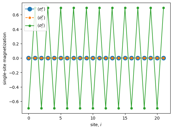
In order to compute the connected spin-spin correlators we first need to compute the magnetization on each site along the three axes.
In order to project qubit operators using qiskit_addon_sqd.qubit.project_operator_to_subspace, the ``bitstring_matrix`` must first be sorted and de-duplicated, or the function will return unexpected results.
[5]:
from qiskit_addon_sqd.qubit import sort_and_remove_duplicates

# NOTE: It is essential for the projection code to have the bitstrings sorted!
bitstring_matrix = sort_and_remove_duplicates(bitstring_matrix)
[6]:
from qiskit.quantum_info import SparsePauliOp
from qiskit_addon_sqd.qubit import project_operator_to_subspace

s_x = np.zeros(num_spins)
s_y = np.zeros(num_spins)
s_z = np.zeros(num_spins)

for i in range(num_spins):
    # Sigma_x
    pstr = ["I" for _ in range(num_spins)]
    pstr[i] = "X"
    pauli_op = SparsePauliOp("".join(pstr))
    sparse_op = project_operator_to_subspace(bitstring_matrix, pauli_op)
    s_x[i] += np.real(np.conjugate(min_eval).T @ sparse_op @ min_eval)

    # Sigma_y
    pstr = ["I" for i in range(num_spins)]
    pstr[i] = "Y"
    pauli_op = SparsePauliOp("".join(pstr))
    sparse_op = project_operator_to_subspace(bitstring_matrix, pauli_op)
    s_y[i] += np.real(np.conjugate(min_eval).T @ sparse_op @ min_eval)

    # Sigma_z
    pstr = ["I" for i in range(num_spins)]
    pstr[i] = "Z"
    pauli_op = SparsePauliOp("".join(pstr))
    sparse_op = project_operator_to_subspace(bitstring_matrix, pauli_op)
    s_z[i] += np.real(np.conjugate(min_eval).T @ sparse_op @ min_eval)
[7]:
import matplotlib.pyplot as plt

plt.plot(s_x, marker=".", markersize=20, label="x")
plt.plot(s_y, marker=".", linestyle="--", markersize=10, label="y")
plt.plot(s_z, marker=".", markersize=10, label="z")

plt.legend(
    [r"$\langle\sigma^x_i\rangle$", r"$\langle\sigma^y_i\rangle$", r"$\langle\sigma^z_i\rangle$"]
)
plt.xlabel("site, $i$")
plt.ylabel("single-site magnetization")
plt.show()
Once we have computed the average magnetization on each site, we can compute the connected correlators as well.
[8]:
max_distance = num_spins // 2

c_x = np.zeros(max_distance)
c_y = np.zeros(max_distance)
c_z = np.zeros(max_distance)
distance_counts = np.zeros(max_distance)

for i in range(num_spins):
    for j in range(i + 1, num_spins):
        j_wrap = j % num_spins  # Connect qubits N and 0
        distance = min([abs(i - j), abs(i + (num_spins - j))])

        # Sigma_x Sigma_x
        pstr = ["I" for _ in range(num_spins)]
        pstr[i] = "X"
        pstr[j_wrap] = "X"
        pauli_op = SparsePauliOp("".join(pstr))
        sparse_op = project_operator_to_subspace(bitstring_matrix, pauli_op)
        c_x[distance - 1] += (
            np.real(np.conjugate(min_eval).T @ sparse_op @ min_eval) - s_x[i] * s_x[j_wrap]
        )

        # Sigma_y Sigma_y
        pstr = ["I" for _ in range(num_spins)]
        pstr[i] = "Y"
        pstr[j_wrap] = "Y"
        pauli_op = SparsePauliOp("".join(pstr))
        sparse_op = project_operator_to_subspace(bitstring_matrix, pauli_op)
        c_y[distance - 1] += (
            np.real(np.conjugate(min_eval).T @ sparse_op @ min_eval) - s_y[i] * s_y[j_wrap]
        )

        # Sigma_z Sigma_z
        pstr = ["I" for _ in range(num_spins)]
        pstr[i] = "Z"
        pstr[j_wrap] = "Z"
        pauli_op = SparsePauliOp("".join(pstr))
        sparse_op = project_operator_to_subspace(bitstring_matrix, pauli_op)
        c_z[distance - 1] += (
            np.real(np.conjugate(min_eval).T @ sparse_op @ min_eval) - s_z[i] * s_z[j_wrap]
        )

        distance_counts[distance - 1] += 1
c_x /= distance_counts
c_y /= distance_counts
c_z /= distance_counts
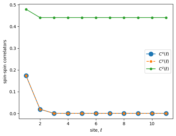
We can see that the Z correlation shows true long range order (the correlator does not decay to 0). The X,Y correlators decay to 0 with distance between spin pairs.
[9]:
plt.plot(np.arange(1, max_distance + 1), np.abs(c_x), marker=".", markersize=20, label="xx")
plt.plot(
    np.arange(1, max_distance + 1),
    np.abs(c_y),
    marker=".",
    linestyle="--",
    markersize=10,
    label="yy",
)
plt.plot(np.arange(1, max_distance + 1), np.abs(c_z), marker=".", markersize=10, label="zz")

plt.legend([r"$C^x(\ell)$", r"$C^y(\ell)$", r"$C^z(\ell)$"])
plt.xlabel(r"site, $\ell$")
plt.ylabel("spin-spin correlators")
plt.show()
References
[1] Robledo-Moreno, Javier, et al. “Chemistry beyond exact solutions on a quantum-centric supercomputer.” arXiv preprint arXiv:2405.05068 (2024).