Improving energy estimation of a Fermionic Hamiltonian with SQD

In this tutorial we implement a Qiskit pattern showing how to post-process noisy quantum samples to find an approximation to the ground state of the \(N_2\) molecule at equilibrium in the 6-31G basis set. We will follow a sample-based quantum diagonalization approach [1] to process samples taken from a 36-qubit quantum circuit. In order to account for the effect of quantum noise, the self-configuration recovery technique is used.

The pattern can be described in four steps:

1. Step 1: Map to quantum problem

   • Generate an ansatz for estimating the ground state

2. Step 2: Optimize the problem

   • Transpile the ansatz for the backend

3. Step 3: Execute experiments

   • Draw samples from the ansatz using the Sampler primitive

4. Step 4: Post-process results

   • Self-consistent configuration recovery loop

     • Post-process the full set of bitstring samples, using prior knowledge of particle number and the average orbital occupancy calculated on the most recent iteration.

     • Probabilistically create batches of subsamples from recovered bitstrings.

     • Project and diagonalize the molecular Hamiltonian over each sampled subspace.

     • Save the minimum ground state energy found across all batches and update the avg orbital occupancy.

For this example, the interacting-electron Hamiltonian takes the generic form:

\[\begin{split}\hat{H} = \sum_{ \substack{pr\\\sigma} } h_{pr} \, \hat{a}^\dagger_{p\sigma} \hat{a}_{r\sigma} + \sum_{ \substack{prqs\\\sigma\tau} } \frac{(pr|qs)}{2} \, \hat{a}^\dagger_{p\sigma} \hat{a}^\dagger_{q\tau} \hat{a}_{s\tau} \hat{a}_{r\sigma}\end{split}\]

\(\hat{a}^\dagger_{p\sigma}\)/\(\hat{a}_{p\sigma}\) are the fermionic creation/annihalation operators associated to the \(p\)-th basis set element and the spin \(\sigma\). \(h_{pr}\) and \((pr|qs)\) are the one- and two-body electronic integrals. These are loaded from an fcidump file with standard chemistry software.

The SQD workflow with self-consistent configuration recovery is depicted in the following diagram.

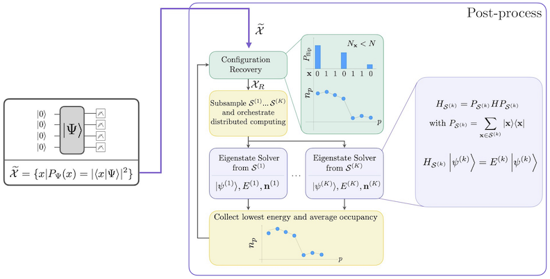
SQD is known to work well when the target eigenstate is sparse: the wave function is supported in a set of basis states \(\mathcal{S} = \{|x\rangle \}\) whose size does not increase exponentially with the size of the problem. In this scenario, the diagonalization of the Hamiltonian projected into the subspace defined by \(\mathcal{S}\):

\[H_\mathcal{S} = P_\mathcal{S} H P_\mathcal{S} \textrm{ with } P_\mathcal{S} = \sum_{x \in \mathcal{S}} |x \rangle \langle x |;\]

yields a good approximation to the target eigenstate. The role of the quantum device is to produce samples of the members of \(\mathcal{S}\) only. First, a quantum circuit prepares the state \(|\Psi\rangle\) in the quantum device. The Jordan-Wigner encoding is used. Consequently, members of the computational basis represent Fock states (electronic configurations/determinants). The circuit is sampled in the computational basis, yielding the set of noisy configurations \(\tilde{\mathcal{X}}\). The configurations are represented by bitstrings. The set \(\tilde{\mathcal{X}}\) is then passed into the classical post-processing block, where the self-consistent configuration recovery technique is used. In the SQD framework, the role of the quantum device is to produce a probability distribution.

Step 1: Map problem to a quantum circuit

In this tutorial, we will approximate the ground state energy of an \(N_2\) molecule. First, we will specify the molecule and its properties. Next, we will create a local unitary cluster Jastrow (LUCJ) ansatz (quantum circuit) to generate samples from a quantum computer for ground state energy estimation.

First, we will specify the molecule and its properties

import warnings

warnings.filterwarnings("ignore")

from pyscf import ao2mo, tools

# Specify molecule properties
num_orbitals = 16
num_elec_a = num_elec_b = 5
open_shell = False
spin_sq = 0

# Read in molecule from disk
mf_as = tools.fcidump.to_scf("../molecules/n2_fci.txt")
hcore = mf_as.get_hcore()
eri = ao2mo.restore(1, mf_as._eri, num_orbitals)
nuclear_repulsion_energy = mf_as.mol.energy_nuc()

Parsing ../molecules/n2_fci.txt

Next, we will create the ansatz. The LUCJ ansatz is a parameterized quantum circuit, and we will initialize it with t2 and t1 amplitudes obtained from a CCSD calculation.

from pyscf import cc

mf_as.kernel()
mc = cc.CCSD(mf_as)
mc.kernel()
t1 = mc.t1
t2 = mc.t2

converged SCF energy = -108.867773675638
E(CCSD) = -109.0935188821144  E_corr = -0.2257452064762984

Overwritten attributes  get_ovlp get_hcore  of <class 'pyscf.scf.hf_symm.SymAdaptedRHF'>

We will use the ffsim package to create and initialize the ansatz with t2 and t1 amplitudes computed above. Since our molecule has a closed-shell Hartree-Fock state, we will use the spin-balanced variant of the UCJ ansatz, UCJOpSpinBalanced.

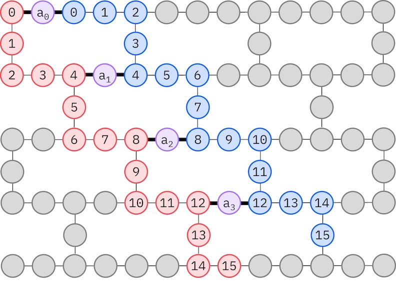
As our target IBM hardware has a heavy-hex topology, we will adopt the zig-zag pattern used in [2] for qubit interactions. In this pattern, orbitals (represented by qubits) with the same spin are connected with a line topology (red and blue circles) where each line take a zig-zag shape due the heavy-hex connectivity of the target hardware. Again, due to the heavy-hex topology, orbitals for different spins have connections between every 4th orbital (0, 4, 8, etc.) (purple circles).

import ffsim
from qiskit import QuantumCircuit, QuantumRegister

n_reps = 2
alpha_alpha_indices = [(p, p + 1) for p in range(num_orbitals - 1)]
alpha_beta_indices = [(p, p) for p in range(0, num_orbitals, 4)]

ucj_op = ffsim.UCJOpSpinBalanced.from_t_amplitudes(
    t2=t2,
    t1=t1,
    n_reps=n_reps,
    interaction_pairs=(alpha_alpha_indices, alpha_beta_indices),
)

nelec = (num_elec_a, num_elec_b)

# create an empty quantum circuit
qubits = QuantumRegister(2 * num_orbitals, name="q")
circuit = QuantumCircuit(qubits)

# prepare Hartree-Fock state as the reference state and append it to the quantum circuit
circuit.append(ffsim.qiskit.PrepareHartreeFockJW(num_orbitals, nelec), qubits)

# apply the UCJ operator to the reference state
circuit.append(ffsim.qiskit.UCJOpSpinBalancedJW(ucj_op), qubits)
circuit.measure_all()

Step 2: Optimize the problem

Next, we will optimize our circuit for a target hardware. We need to choose the hardware device to use before optimizing our circuit. We will use a fake 127-qubit backend from qiskit_ibm_runtime to emulate a real device.

from qiskit_ibm_runtime.fake_provider import FakeSherbrooke

backend = FakeSherbrooke()

Next, we recommend the following steps to optimize the ansatz and make it hardware-compatible.

• Select physical qubits (initial_layout) from the target hardware that adheres to the zig-zag pattern described above. Laying out qubits in this pattern leads to an efficient hardware-compatible circuit with less gates.

• Generate a staged pass manager using the generate_preset_pass_manager function from qiskit with your choice of backend and initial_layout.

• Set the pre_init stage of your staged pass manager to ffsim.qiskit.PRE_INIT. ffsim.qiskit.PRE_INIT includes qiskit transpiler passes that decompose gates into orbital rotations and then merges the orbital rotations, resulting in fewer gates in the final circuit.

• Run the pass manager on your circuit.

from qiskit.transpiler.preset_passmanagers import generate_preset_pass_manager

spin_a_layout = [0, 14, 18, 19, 20, 33, 39, 40, 41, 53, 60, 61, 62, 72, 81, 82]
spin_b_layout = [2, 3, 4, 15, 22, 23, 24, 34, 43, 44, 45, 54, 64, 65, 66, 73]
initial_layout = spin_a_layout + spin_b_layout

pass_manager = generate_preset_pass_manager(
    optimization_level=3, backend=backend, initial_layout=initial_layout
)

# without PRE_INIT passes
isa_circuit = pass_manager.run(circuit)
print(f"Gate counts (w/o pre-init passes): {isa_circuit.count_ops()}")

# with PRE_INIT passes
# We will use the circuit generated by this pass manager for hardware execution
pass_manager.pre_init = ffsim.qiskit.PRE_INIT
isa_circuit = pass_manager.run(circuit)
print(f"Gate counts (w/ pre-init passes): {isa_circuit.count_ops()}")

Gate counts (w/o pre-init passes): OrderedDict({'rz': 7419, 'sx': 6016, 'ecr': 2240, 'x': 323, 'measure': 32, 'barrier': 1})
Gate counts (w/ pre-init passes): OrderedDict({'rz': 4158, 'sx': 3186, 'ecr': 1262, 'x': 210, 'measure': 32, 'barrier': 1})

Step 3: Execute experiments

After optimizing the circuit for hardware execution, we are ready to run it on the target hardware and collect samples for ground state energy estimation. As we only have one circuit, we will use Qiskit Runtime’s Job execution mode and execute our circuit.

Note: We have commented out the code for running the circuit on a QPU and left it for the user’s reference. Instead of running on real hardware in this guide, we will just generate random samples drawn from the uniform distribution.

# from qiskit_ibm_runtime import SamplerV2 as Sampler

# sampler = Sampler(mode=backend)
# job = sampler.run([isa_circuit], shots=10_000)
# primitive_result = job.result()
# pub_result = primitive_result[0]
# counts = pub_result.data.meas.get_counts()

from qiskit_addon_sqd.counts import generate_counts_uniform

rand_seed = 42
counts = generate_counts_uniform(10_000, num_orbitals * 2, rand_seed=rand_seed)

Step 4: Post-process results

First, we will transform the counts into a bitstring matrix and probability array for post-processing.

Each row in the matrix represents one unique bitstring. Since qubits are indexed from the right of a bitstring in Qiskit, column 0 represents qubit N-1, and column N-1 represents qubit 0, where N is the number of qubits.

The alpha particles are represented in the column index range (N, N/2], and the beta particles are represented in the column range (N/2, 0].

import numpy as np
from qiskit_addon_sqd.counts import counts_to_arrays

# Convert counts into bitstring and probability arrays
bitstring_matrix_full, probs_arr_full = counts_to_arrays(counts)

Iteratively refine the samples using configuration recovery and approximate the ground state at each iteration

There are a few user-controlled options which are important for this technique:

• iterations: Number of self-consistent configuration recovery iterations

• n_batches: Number of batches of configurations used by the different calls to the eigenstate solver

• samples_per_batch: Number of unique configurations to include in each batch

• max_davidson_cycles: Maximum number of Davidson cycles run by each eigensolver

from qiskit_addon_sqd.configuration_recovery import recover_configurations
from qiskit_addon_sqd.fermion import (
    flip_orbital_occupancies,
    solve_fermion,
)
from qiskit_addon_sqd.subsampling import postselect_and_subsample

# SQD options
iterations = 5

# Eigenstate solver options
n_batches = 10
samples_per_batch = 300
max_davidson_cycles = 200

# Self-consistent configuration recovery loop
e_hist = np.zeros((iterations, n_batches))  # energy history
s_hist = np.zeros((iterations, n_batches))  # spin history
occupancy_hist = np.zeros((iterations, 2 * num_orbitals))
occupancies_bitwise = None  # orbital i corresponds to column i in bitstring matrix
for i in range(iterations):
    print(f"Starting configuration recovery iteration {i}")
    # On the first iteration, we have no orbital occupancy information from the
    # solver, so we just post-select from the full bitstring set based on hamming weight.
    if occupancies_bitwise is None:
        bs_mat_tmp = bitstring_matrix_full
        probs_arr_tmp = probs_arr_full

    # If we have average orbital occupancy information, we use it to refine the full set of noisy configurations
    else:
        bs_mat_tmp, probs_arr_tmp = recover_configurations(
            bitstring_matrix_full,
            probs_arr_full,
            occupancies_bitwise,
            num_elec_a,
            num_elec_b,
            rand_seed=rand_seed,
        )

    # Throw out configurations with incorrect particle number in either the spin-up or spin-down systems
    batches = postselect_and_subsample(
        bs_mat_tmp,
        probs_arr_tmp,
        hamming_right=num_elec_a,
        hamming_left=num_elec_b,
        samples_per_batch=samples_per_batch,
        num_batches=n_batches,
        rand_seed=rand_seed,
    )

    # Run eigenstate solvers in a loop. This loop should be parallelized for larger problems.
    e_tmp = np.zeros(n_batches)
    s_tmp = np.zeros(n_batches)
    occs_tmp = np.zeros((n_batches, 2 * num_orbitals))
    coeffs = []
    for j in range(n_batches):
        energy_sci, coeffs_sci, avg_occs, spin = solve_fermion(
            batches[j],
            hcore,
            eri,
            open_shell=open_shell,
            spin_sq=spin_sq,
            max_davidson=max_davidson_cycles,
        )
        energy_sci += nuclear_repulsion_energy
        e_tmp[j] = energy_sci
        s_tmp[j] = spin
        occs_tmp[j, :num_orbitals] = avg_occs[0]
        occs_tmp[j, num_orbitals:] = avg_occs[1]
        coeffs.append(coeffs_sci)

    # Combine batch results
    avg_occupancy = np.mean(occs_tmp, axis=0)
    # The occupancies from the solver should be flipped to match the bits in the bitstring matrix.
    occupancies_bitwise = flip_orbital_occupancies(avg_occupancy)

    # Track optimization history
    e_hist[i, :] = e_tmp
    s_hist[i, :] = s_tmp
    occupancy_hist[i, :] = avg_occupancy

Starting configuration recovery iteration 0
Starting configuration recovery iteration 1
Starting configuration recovery iteration 2
Starting configuration recovery iteration 3
Starting configuration recovery iteration 4

Visualize the results

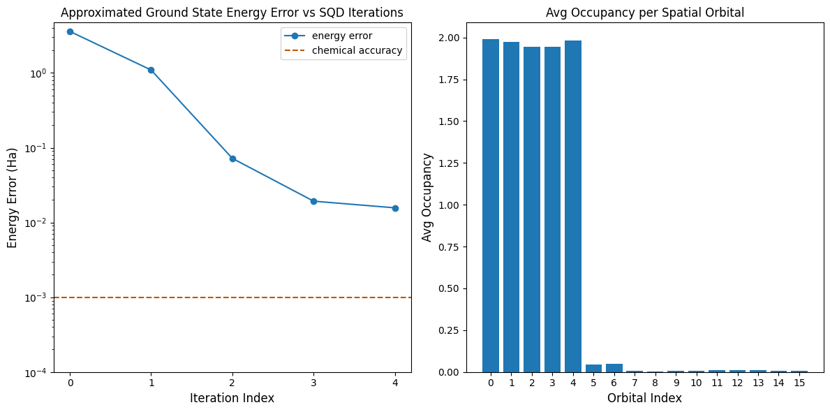
The first plot shows that after a couple of iterations we estimate the ground state energy within ~200 mH (chemical accuracy is typically accepted to be 1 kcal/mol \(\approx\) 1.6 mH). Remember, the quantum samples in this demo were pure noise. The signal here comes from a priori knowledge of the electronic structure and molecular Hamiltonian.

The second plot shows the average occupancy of each spatial orbital after the final iteration. We can see that both the spin-up and spin-down electrons occupy the first five orbitals with high probability in our solutions.

import matplotlib.pyplot as plt

# Data for energies plot
n2_exact = -109.10288938
x1 = range(iterations)
e_diff = [abs(np.min(energies) - n2_exact) for energies in e_hist]
yt1 = [1.0, 1e-1, 1e-2, 1e-3, 1e-4]

# Chemical accuracy (+/- 1 milli-Hartree)
chem_accuracy = 0.001

# Data for avg spatial orbital occupancy
y2 = avg_occupancy[:num_orbitals] + avg_occupancy[num_orbitals:]
x2 = range(len(y2))

fig, axs = plt.subplots(1, 2, figsize=(12, 6))

# Plot energies
axs[0].plot(x1, e_diff, label="energy error", marker="o")
axs[0].set_xticks(x1)
axs[0].set_xticklabels(x1)
axs[0].set_yticks(yt1)
axs[0].set_yticklabels(yt1)
axs[0].set_yscale("log")
axs[0].set_ylim(1e-4)
axs[0].axhline(y=chem_accuracy, color="#BF5700", linestyle="--", label="chemical accuracy")
axs[0].set_title("Approximated Ground State Energy vs SQD Iterations")
axs[0].set_xlabel("Iteration Index", fontdict={"fontsize": 12})
axs[0].set_ylabel("Energy Error (Ha)", fontdict={"fontsize": 12})
axs[0].legend()

# Plot orbital occupancy
axs[1].bar(x2, y2, width=0.8)
axs[1].set_xticks(x2)
axs[1].set_xticklabels(x2)
axs[1].set_title("Avg Occupancy per Spatial Orbital")
axs[1].set_xlabel("Orbital Index", fontdict={"fontsize": 12})
axs[1].set_ylabel("Avg Occupancy", fontdict={"fontsize": 12})

plt.tight_layout()
plt.show()

References

[1] Robledo-Moreno, Javier, et al. “Chemistry beyond exact solutions on a quantum-centric supercomputer.” arXiv preprint arXiv:2405.05068 (2024).

[2] Motta, Mario, et al. “Bridging physical intuition and hardware efficiency for correlated electronic states: the local unitary cluster Jastrow ansatz for electronic structure.” Chemical Science 14.40 (2023): 11213-11227.