Improving energy estimation of a Fermionic lattice model with SQD
In this tutorial we implement a Qiskit pattern showing how to post-process noisy quantum samples to find an approximation to the ground state of a Fermionic lattice Hamiltonian known as the single-impurity Anderson model. We will follow a sample-based quantum diagonalization approach to process samples taken from a set of 16-qubit Krylov basis states over increasing time intervals. These states are realized on the quantum
device using Trotterization of the time evolution. In order to account for the effect of quantum noise, the configuration recovery technique is used. Assuming a good initial state and sparsity of the ground state, this approach is proven to converge efficiently.
The pattern can be described in four steps:
Step 1: Map to quantum problem
Generate a set of Krylov basis states (i.e., Trotterized time-evolution circuits) over increasing time intervals for estimating the ground state
Step 2: Optimize the problem
Transpile the circuits for the backend
Step 3: Execute experiments
Draw samples from the circuits using the
Samplerprimitive
Step 4: Post-process results
Self-consistent configuration recovery loop
Post-process the full set of bitstring samples, using prior knowledge of particle number and the average orbital occupancy calculated on the most recent iteration
Probabilistically create batches of subsamples from recovered bitstrings
Project and diagonalize the Fermionic lattice Hamiltonian over each sampled subspace
Save the minimum ground state energy found across all batches and update the avg orbital occupancy
Step 1: Map problem to a quantum circuit
First, we will create the one- and two-body Hamiltonians describing the one-dimensional single-impurity Anderson model (SIAM) with 7 bath sites (8 electrons in 8 orbitals). This model is used to describe magnetic impurities embedded in metals.
Then we will create the 16-qubit Trotter circuits used to generate the quantum Krylov subspace.
[1]:
import numpy as np

n_bath = 7  # number of bath sites

V = 1  # hybridization amplitude
t = 1  # bath hopping amplitude
U = 10  # Impurity onsite repulsion
eps = -U / 2  # Chemical potential for the impurity

# Place the impurity on the first qubit
impurity_index = 0

# One body matrix elements in the "position" basis
h1e = -t * np.diag(np.ones(n_bath), k=1) - t * np.diag(np.ones(n_bath), k=-1)
h1e[impurity_index, impurity_index + 1] = -V
h1e[impurity_index + 1, impurity_index] = -V
h1e[impurity_index, impurity_index] = eps

# Two body matrix elements in the "position" basis
h2e = np.zeros((n_bath + 1, n_bath + 1, n_bath + 1, n_bath + 1))
h2e[impurity_index, impurity_index, impurity_index, impurity_index] = U
Next, we will generate the quantum Krylov subspace with a set of Trotterized quantum circuits. Here we create helpers for generating the initial (reference) state as well as the time evolution for the one- and two-body parts of the Hamiltonian. For a more detailed description of this model and how the circuits are designed, please refer to the paper.
[2]:
import ffsim
import scipy
from qiskit import QuantumCircuit, QuantumRegister
from qiskit.circuit.library import CPhaseGate, XGate, XXPlusYYGate

n_modes = n_bath + 1
nelec = (n_modes // 2, n_modes // 2)

dt = 0.2
Utar = scipy.linalg.expm(-1j * dt * h1e)


# The reference state
def initial_state(q_circuit, norb, nocc):
    """Prepare an initial state."""
    for i in range(nocc):
        q_circuit.append(XGate(), [i])
        q_circuit.append(XGate(), [norb + i])
    rot = XXPlusYYGate(np.pi / 2, -np.pi / 2)

    for i in range(3):
        for j in range(nocc - i - 1, nocc + i, 2):
            q_circuit.append(rot, [j, j + 1])
            q_circuit.append(rot, [norb + j, norb + j + 1])
    q_circuit.append(rot, [j + 1, j + 2])
    q_circuit.append(rot, [norb + j + 1, norb + j + 2])


# The one-body time evolution
free_fermion_evolution = ffsim.qiskit.OrbitalRotationJW(n_modes, Utar)


# The two-body time evolution
def append_diagonal_evolution(dt, U, impurity_qubit, num_orb, q_circuit):
    """Append two-body time evolution to a quantum circuit."""
    if U != 0:
        q_circuit.append(
            CPhaseGate(-dt / 2 * U),
            [impurity_qubit, impurity_qubit + num_orb],
        )
Generate d time-evolved states that specify the quantum Krylov subspace. Here, we have chosen d=8. The error from sampling Krylov basis states converges with increasing d. Note that the particulars of this problem instance allow for an efficient compilation of the one-body evolution using OrbitalRotationJW; however, in general, one could use Qiskit’s PauliEvolutionGate to implement the
Trotterized time evolution of the full Hamiltonian.
[3]:
# Generate the initial state
qubits = QuantumRegister(2 * n_modes, name="q")
init_state = QuantumCircuit(qubits)
initial_state(init_state, n_modes, n_modes // 2)
init_state.draw("mpl", scale=0.4, fold=-1)

d = 8  # Number of Krylov basis states
circuits = []
for i in range(d):
    circ = init_state.copy()
    circuits.append(circ)
    for _ in range(i):
        append_diagonal_evolution(dt, U, impurity_index, n_modes, circ)
        circ.append(free_fermion_evolution, qubits)
        append_diagonal_evolution(dt, U, impurity_index, n_modes, circ)
    circ.measure_all()
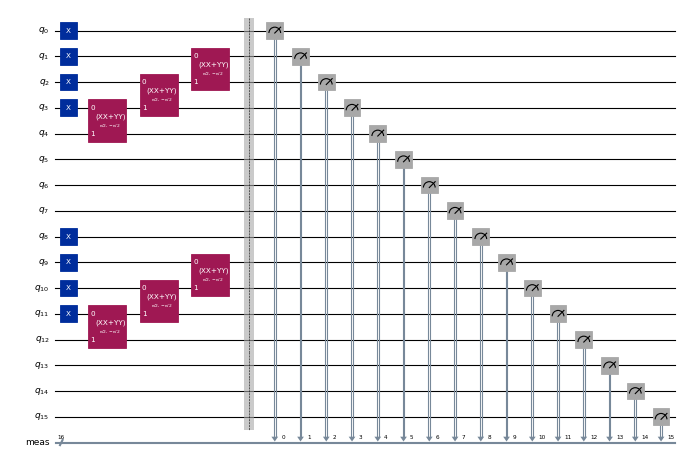
[4]:
circuits[0].draw("mpl", scale=0.4, fold=-1)
[4]:
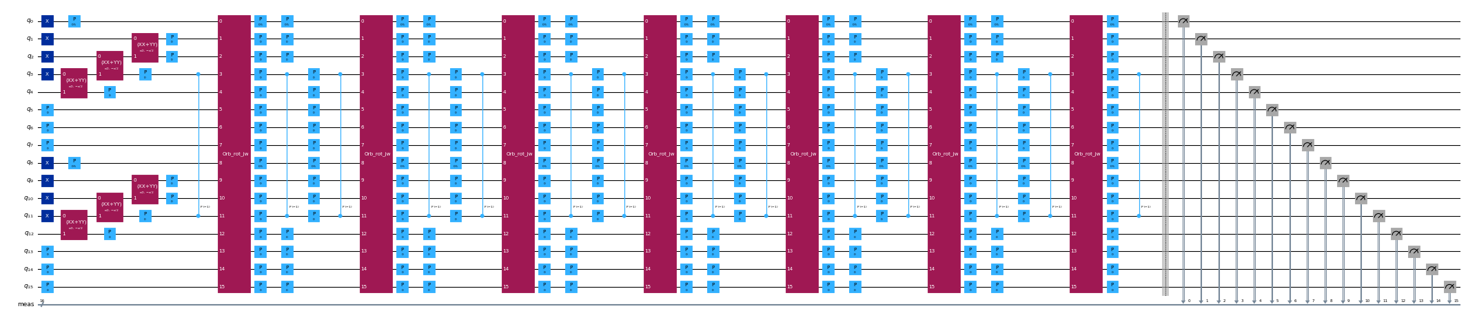
[5]:
circuits[-1].draw("mpl", scale=0.4, fold=-1)
[5]:
Step 2: Optimize the problem
After we have created the Trotterized circuits, we will optimize them for a target hardware. We need to choose the hardware device to use before optimization. We will use a fake 127-qubit backend from qiskit_ibm_runtime to emulate a real device. To run on a real QPU, just replace the fake backend with a real backend. Check out the Qiskit IBM Runtime docs for more info.
[6]:
from qiskit_ibm_runtime.fake_provider.backends import FakeSherbrooke

backend = FakeSherbrooke()
Next, we will transpile the circuits to the target backend using Qiskit.
[7]:
from qiskit.transpiler import generate_preset_pass_manager

# The circuit needs to be transpiled to the AerSimulator target
pass_manager = generate_preset_pass_manager(optimization_level=3, backend=backend)
isa_circuits = pass_manager.run(circuits)
Step 3: Execute experiments
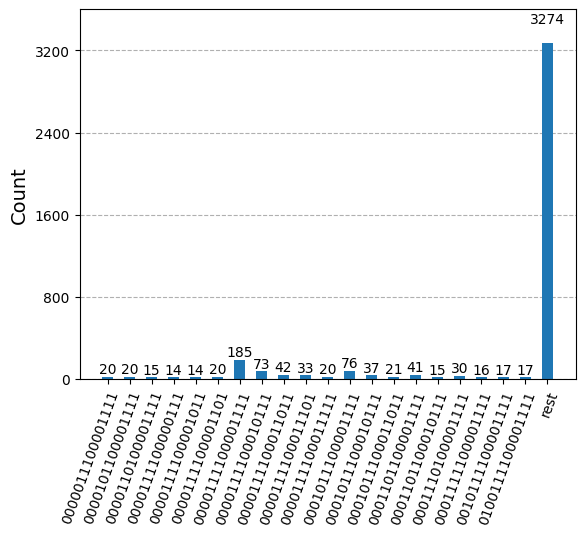
After optimizing the circuits for hardware execution, we are ready to run them on the target hardware and collect samples for ground state energy estimation. Here we use SamplerV2 from qiskit-ibm-runtime to simulate noisy samples taken from the ibm_sherbrooke backend. We then combine the counts from each of the Krylov basis states into a single counts dictionary and plot the top 20 most commonly sampled bitstrings.
Note: Qiskit Aer is required to simulate samples from transpiled circuits.
[8]:
from qiskit.primitives import BitArray
from qiskit.visualization import plot_histogram
from qiskit_ibm_runtime import SamplerV2 as Sampler

# Sample from the circuits
noisy_sampler = Sampler(backend, options={"simulator": {"seed_simulator": 24}})
job = noisy_sampler.run(isa_circuits, shots=500)

# Combine the counts from the individual Trotter circuits
bit_array = BitArray.concatenate_shots([result.data.meas for result in job.result()])

plot_histogram(bit_array.get_counts(), number_to_keep=20)
[8]:
Step 4: Post-process the results
Now, we run the SQD algorithm using the diagonalize_fermionic_hamiltonian function. See the API documentation for explanations of the arguments to this function.
[ ]:
from qiskit_addon_sqd.fermion import SCIResult, diagonalize_fermionic_hamiltonian

# List to capture intermediate results
result_history = []


def callback(results: list[SCIResult]):
    result_history.append(results)
    iteration = len(result_history)
    print(f"Iteration {iteration}")
    for i, result in enumerate(results):
        print(f"\tSubsample {i}")
        print(f"\t\tEnergy: {result.energy}")
        print(f"\t\tSubspace dimension: {np.prod(result.sci_state.amplitudes.shape)}")


rng = np.random.default_rng(24)
result = diagonalize_fermionic_hamiltonian(
    h1e,
    h2e,
    bit_array,
    samples_per_batch=300,
    norb=n_modes,
    nelec=nelec,
    num_batches=3,
    max_iterations=10,
    symmetrize_spin=True,
    callback=callback,
    seed=rng,
)
Iteration 1
        Subsample 0
                Energy: -13.257128325607997
                Subspace dimension: 3969
        Subsample 1
                Energy: -13.257128325607997
                Subspace dimension: 3969
        Subsample 2
                Energy: -13.257128325607997
                Subspace dimension: 3969
Iteration 2
        Subsample 0
                Energy: -13.319666127542039
                Subspace dimension: 4096
        Subsample 1
                Energy: -13.420534292304595
                Subspace dimension: 4624
        Subsample 2
                Energy: -9.136171594591085
                Subspace dimension: 4624
Iteration 3
        Subsample 0
                Energy: -13.422491814612833
                Subspace dimension: 4900
        Subsample 1
                Energy: -13.422491814612833
                Subspace dimension: 4900
        Subsample 2
                Energy: -13.422491814612833
                Subspace dimension: 4900
Iteration 4
        Subsample 0
                Energy: -13.422491814612833
                Subspace dimension: 4900
        Subsample 1
                Energy: -13.422491814612833
                Subspace dimension: 4900
        Subsample 2
                Energy: -13.422491814612833
                Subspace dimension: 4900
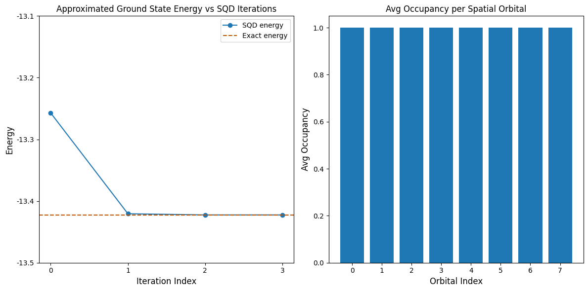
Now, we plot the results. The first plot shows that after a few iterations, we obtain the exact ground state energy.
This example is small enough that we are able to explore the full Hilbert space, as seen in the print statements above. Remember, the full Hilbert space is dimension (num_orbitals choose nelec_a) * (num_orbitals choose nelec_b). So for this problem: (8 choose 4)**2 = 4900. The subspace dimensions increase due enhanced configuration recovery, and also the fact that the SQD algorithm carries important configurations from one iteration to the next. By the last iteration, we are
diagonalizing in the entire Hilbert space.
The second plot shows the average occupancy of each spatial orbital across all batches’ solutions. We see that with high probability each orbital contains one electron.
[10]:
import matplotlib.pyplot as plt

exact_energy = -13.422491814605827
min_es = [min(result, key=lambda res: res.energy).energy for result in result_history]
min_id, min_e = min(enumerate(min_es), key=lambda x: x[1])

# Data for energies plot
x1 = range(len(result_history))
yt1 = list(np.arange(-13.5, -13.1, 0.1))
ytl = [f"{i:.1f}" for i in yt1]

# Data for avg spatial orbital occupancy
y2 = np.sum(result.orbital_occupancies, axis=0)
x2 = range(len(y2))

fig, axs = plt.subplots(1, 2, figsize=(12, 6))

# Plot energies
axs[0].plot(x1, min_es, label="SQD energy", marker="o")
axs[0].set_xticks(x1)
axs[0].set_xticklabels(x1)
axs[0].set_yticks(yt1)
axs[0].set_yticklabels(ytl)
axs[0].axhline(y=exact_energy, color="#BF5700", linestyle="--", label="Exact energy")
axs[0].set_title("Approximated Ground State Energy vs SQD Iterations")
axs[0].set_xlabel("Iteration Index", fontdict={"fontsize": 12})
axs[0].set_ylabel("Energy", fontdict={"fontsize": 12})
axs[0].legend()

# Plot orbital occupancy
axs[1].bar(x2, y2, width=0.8)
axs[1].set_xticks(x2)
axs[1].set_xticklabels(x2)
axs[1].set_title("Avg Occupancy per Spatial Orbital")
axs[1].set_xlabel("Orbital Index", fontdict={"fontsize": 12})
axs[1].set_ylabel("Avg Occupancy", fontdict={"fontsize": 12})

print(f"Exact energy: {exact_energy:.5f}")
print(f"SQD energy: {min_e:.5f}")
print(f"Absolute error: {abs(min_e - exact_energy):.5f}")
plt.tight_layout()
plt.show()
Exact energy: -13.42249
SQD energy: -13.42249
Absolute error: 0.00000