How to place wire cuts using a single-qubit `CutWire` instruction¶

This how-to guide is intended to demonstrate how to place wire cuts using single-qubit CutWire instructions, which may at times be more convenient than specifying them as two-qubit Move instructions.

[1]:

import numpy as np
from qiskit import QuantumCircuit
from qiskit.quantum_info import SparsePauliOp
from qiskit_aer.primitives import EstimatorV2, SamplerV2

from qiskit_addon_cutting import (
    partition_problem,
    generate_cutting_experiments,
    reconstruct_expectation_values,
)

from qiskit_addon_cutting.instructions import CutWire
from qiskit_addon_cutting import cut_wires, expand_observables

Prepare a circuit for cutting¶

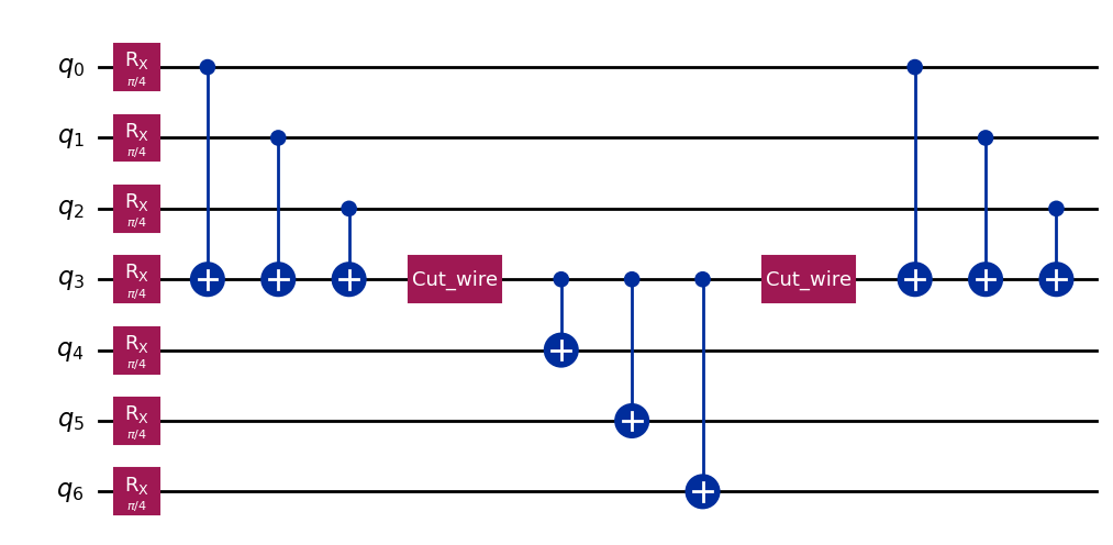
As in the tutorial for wire cutting, we have used a circuit inspired by Fig. 1(a) of arXiv:2302.03366v1. The cut locations are marked manually here with CutWire instructions.

[2]:

qc_0 = QuantumCircuit(7)
for i in range(7):
    qc_0.rx(np.pi / 4, i)
qc_0.cx(0, 3)
qc_0.cx(1, 3)
qc_0.cx(2, 3)
qc_0.append(CutWire(), [3])
qc_0.cx(3, 4)
qc_0.cx(3, 5)
qc_0.cx(3, 6)
qc_0.append(CutWire(), [3])
qc_0.cx(0, 3)
qc_0.cx(1, 3)
qc_0.cx(2, 3)
qc_0.draw("mpl")

[2]:

../_images/how-tos_how_to_specify_cut_wires_3_0.png

Recover the uncut circuit¶

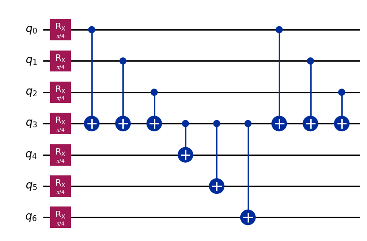
CutWire instructions decompose to nothing (they are equivalent to the identity), so the uncut circuit can be recovered as follows:

[3]:

qc_0.decompose("cut_wire").draw("mpl")

[3]:

../_images/how-tos_how_to_specify_cut_wires_5_0.png

Specify an observable¶

This observable has 7 qubits, just like the original circuit.

[4]:

observable = SparsePauliOp(["ZIIIIII", "IIIZIII", "IIIIIIZ"])

Transform cuts to moves¶

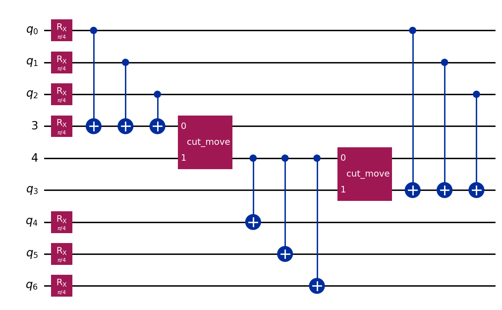
The next step is to call cut_wires, which transforms each CutWire into a TwoQubitQPDGate which wraps a Move instruction. An additional qubit is added to the circuit for each CutWire in the input circuit.

Notice that, unlike in the wire cutting tutorial, where Move operations were placed manually, this function does not result in the re-use of a qubit. Because any method for qubit re-use is based on heuristics, this function naively allocates an additional qubit for each cut. Users wishing to re-use qubits might wish to experiment with qiskit-qubit-reuse.

[5]:

qc_1 = cut_wires(qc_0)
qc_1.draw("mpl")

[5]:

../_images/how-tos_how_to_specify_cut_wires_9_0.png

Update the observable terms to account for the extra qubit¶

The transformed circuit contains additional qubits (one for each CutWire instruction), so the observables must be updated for the new circuit. This can be done using the expand_observables function. Since the observable coefficients are ignored until reconstruction of the final expectation value, the input and output types of the observables for expand_observables are PauliLists.

The resulting observables have 9 qubits, just like the transformed circuit.

[6]:

observable_expanded_paulis = expand_observables(observable.paulis, qc_0, qc_1)
observable_expanded_paulis

[6]:

PauliList(['ZIIIIIIII', 'IIIZIIIII', 'IIIIIIIIZ'])

Separate the circuit and observables¶

In this case, partition_labels need not be passed to partition_problem, as the labels can be determined automatically from the connectivity of the circuit.

[7]:

partitioned_problem = partition_problem(
    circuit=qc_1, observables=observable_expanded_paulis
)
subcircuits = partitioned_problem.subcircuits
subobservables = partitioned_problem.subobservables

From here forward, the cutting workflow is the same as usual, but the remaining steps are spelled out here explicitly so one can follow along with the results.

Visualize the decomposed problem¶

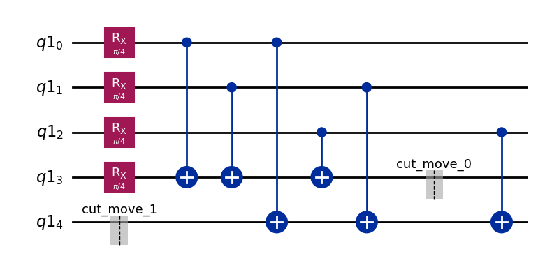
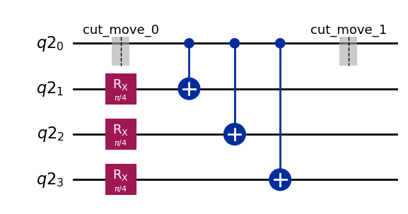
Notice that once the circuits have been cut, some of the instructions are able to commute past each other. For instance, in subcircuit “A”, half of the second Move operation is actually the first operation on the final qubit.

[8]:

subobservables

[8]:

{0: PauliList(['IIIII', 'ZIIII', 'IIIIZ']),
 1: PauliList(['ZIII', 'IIII', 'IIII'])}

[9]:

subcircuits[0].draw("mpl")

[9]:

../_images/how-tos_how_to_specify_cut_wires_17_0.png

[10]:

subcircuits[1].draw("mpl")

[10]:

../_images/how-tos_how_to_specify_cut_wires_18_0.png

Generate and run the cutting experiments; reconstruct and compare against uncut expectation values¶

[11]:

subexperiments, coefficients = generate_cutting_experiments(
    circuits=subcircuits,
    observables=subobservables,
    num_samples=np.inf,
)

[12]:

sampler = SamplerV2()
results = {
    label: sampler.run(subexperiment, shots=2**12).result()
    for label, subexperiment in subexperiments.items()
}

[13]:

reconstructed_expval_terms = reconstruct_expectation_values(
    results,
    coefficients,
    subobservables,
)
reconstructed_expval = np.dot(reconstructed_expval_terms, observable.coeffs)

[14]:

estimator = EstimatorV2()
exact_expval = (
    estimator.run([(qc_0.decompose("cut_wire"), observable)]).result()[0].data.evs
)
print(f"Reconstructed expectation value: {np.real(np.round(reconstructed_expval, 8))}")
print(f"Exact expectation value: {np.round(exact_expval, 8)}")
print(f"Error in estimation: {np.real(np.round(reconstructed_expval-exact_expval, 8))}")
print(
    f"Relative error in estimation: {np.real(np.round((reconstructed_expval-exact_expval) / exact_expval, 8))}"
)

Reconstructed expectation value: 1.63000017
Exact expectation value: 1.59099026
Error in estimation: 0.03900992
Relative error in estimation: 0.02451927

How to place wire cuts using a single-qubit CutWire instruction¶