Optimization Solver: A Qiskit Function by Q-CTRL Fire Opal
See the API reference
Qiskit Functions are an experimental feature available only to IBM Quantum® Premium Plan, Flex Plan, and On-Prem (via IBM Quantum Platform API) Plan users. They are in preview release status and subject to change.
Overview
With the Fire Opal Optimization Solver, you can solve utility-scale optimization problems on quantum hardware without requiring quantum expertise. Simply input the high-level problem definition, and the Solver takes care of the rest. The entire workflow is noise-aware and leverages Fire Opal's Performance Management under the hood. The Solver consistently delivers accurate solutions to classically challenging problems, even at full-device scale on the largest IBM® QPUs.
The Solver is flexible and can be used to solve combinatorial optimization problems defined as objective functions or arbitrary graphs. Problems do not have to be mapped to device topology. Both unconstrained and constrained problems are solvable, with constraints enforced as hard Hamming-weight-1 constraints rather than penalty terms. The examples included in this guide demonstrate how to solve an unconstrained and a constrained utility-scale optimization problem using different Solver input types. The first example involves a max-cut problem defined on a 156-node, 3-Regular graph, while the second example tackles a 50-node graph partitioning problem defined by a cost function.
To get access to the Optimization Solver, contact Q-CTRL.
Function description
The Solver fully optimizes and automates the entire algorithm, from error suppression at the hardware level to efficient problem mapping and closed-loop classical optimization. Behind the scenes, the Solver's pipeline reduces errors at every stage, enabling the enhanced performance required to meaningfully scale. The underlying workflow is inspired by the Quantum Approximate Optimization Algorithm (QAOA), which is a hybrid quantum-classical algorithm. For a detailed summary of the full Optimization Solver workflow, refer to the published manuscript.
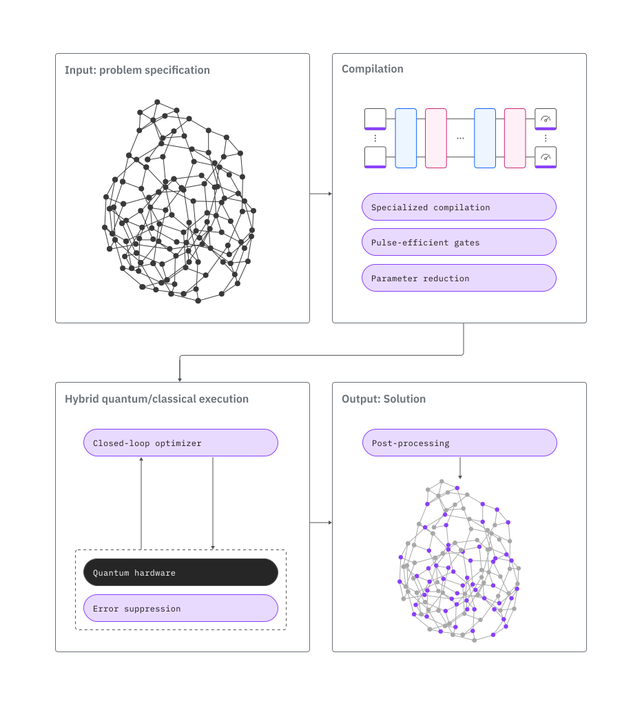
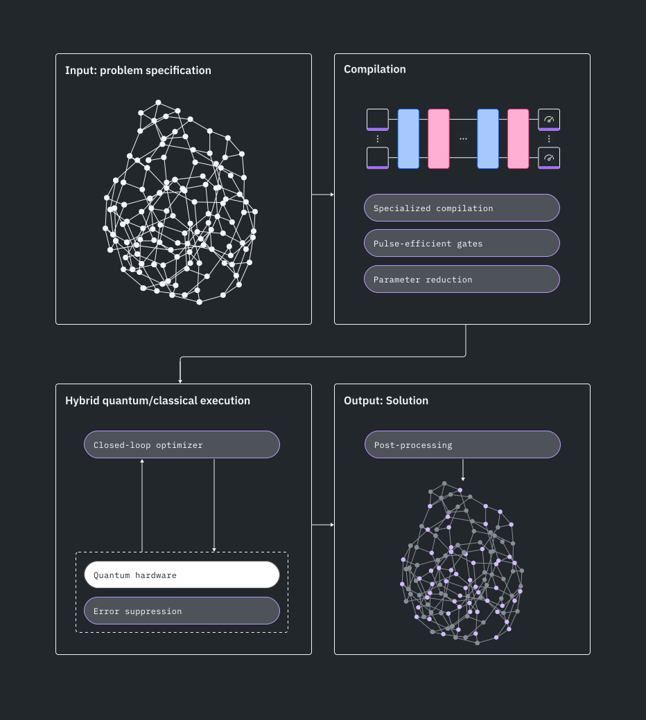
To solve a generic problem with the Optimization Solver:
- Define your problem as an objective function, a graph, or
SparsePauliOpspin chain. - Connect to the function through the Qiskit Functions Catalog.
- Run the problem with the Solver and retrieve results.
Accepted problem formats
- Polynomial expression representation of an objective function. Ideally created in Python with an existing SymPy Poly object and formatted into a string using sympy.srepr.
- Graph representation of a specific problem type. The graph should be created using the networkx library in Python. It should then converted to a string by using the networkx function
nx.readwrite.json_graph.adjacency_data. - Spin chain representation of a specific problem. The spin chain should be represented as a
SparsePauliOpobject; see the documentation for more details.
If you want to use a backend that this function does not currently support, reach out to Q-CTRL to add support.
Benchmarks
Performance can depend on both the problem instance and subsequent processing steps. In some cases, classical samples and quantum-generated samples might achieve similar final solution quality after equivalent post-processing. Evaluation should therefore consider the complete optimization workflow.
Published benchmarking results show that the Solver successfully solves problems with over 120 qubits, even outperforming previously published results on quantum annealing and trapped-ion devices. The following benchmark metrics provide a rough indication of the accuracy and scaling of problem types based on a few examples. Actual metrics may differ based on various problem features, such as the number of terms in the objective function (density) and their locality, number of variables, and polynomial order.
The "Number of qubits" indicated is not a hard limitation but represents rough thresholds where you can expect extremely consistent solution accuracy. Larger problem sizes have been successfully solved, and testing beyond these limits is encouraged.
Arbitrary qubit connectivity is supported across all problem types.
Problem type | Number of qubits | Example | Accuracy | Total time (s) | Runtime usage (s) | Number of iterations |
|---|---|---|---|---|---|---|
| Sparsely-connected quadratic problems | 156 | 3-regular max-cut | 100% | 1764 | 293 | 16 |
| Higher-order binary optimization | 156 | Ising spin-glass model | 100% | 1461 | 272 | 16 |
| Densely-connected quadratic problems | 50 | Fully-connected max-cut | 100% | 1758 | 268 | 12 |
| Constrained problem with hard constraints | 50 | Weighted graph partitioning with 8% edge density | 100% | 1074 | 215 | 10 |
Get started
To learn how to load the function and run it, see Get started with Q-CTRL Optimization Solver.
Get support
For any questions or issues, reach out to Q-CTRL.
Next steps
- Request access to Q-CTRL Optimization Solver.
- Visit the API reference for this Qiskit Function.
- Try the Solve higher-order binary optimization problems with Q-CTRL's Optimization Solver tutorial.
- Review Sachdeva, N., et al. (2024). Quantum optimization using a 127-qubit gate-model IBM quantum computer can outperform quantum annealers for nontrivial binary optimization problems. arXiv preprint arXiv:2406.01743.
- Review Loco, D., et al. (2026). Practical protein-pocket hydration-site prediction for drug discovery on a quantum computer. arXiv preprint arXiv:2512.08390.
- Review the Mazda case study.
- Review the Network Rail case study.
- Review the Australian Army case study.
- Review the Transport for New South Wales case study.