Operator backpropagation (OBP) for estimation of expectation values

Usage estimate: 4 minutes on a Heron r3 processor (NOTE: This is an estimate only. Your runtime might vary.)

Learning outcomes

After going through this tutorial, users should understand:

• How to use qiskit-addon-obp to reduce the depth of the quantum circuit at the cost of an increased number of circuit executions
• How to use qiskit-addon-utils to construct XYZ Hamiltonians and their time-evolution circuits

Prerequisites

We suggest that users are familiar with the following topics before going through this tutorial:

• Using the Estimator primitive to calculate expectation values of an observable

Background

Operator backpropagation is a technique that involves absorbing operations from the end of a quantum circuit into the measured observable, generally reducing the depth of the circuit at the cost of additional terms in the observable. The goal is to backpropagate as much of the circuit as possible without allowing the observable to grow too large. A Qiskit-based implementation is available in the OBP Qiskit addon. Read the corresponding documentation for more information.

Consider an example circuit for which an observable $O = \sum_P c_P P$ is to be measured, where $P$ are Paulis and $c_P$ are coefficients. Let us denote the circuit as a single unitary $U$, which can be logically partitioned into $U = U_C U_Q$ as shown in the figure below.

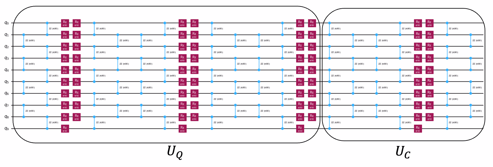
Operator backpropagation absorbs the unitary $U_C$ into the observable by evolving it as $O' = U_C^{\dagger}OU_C = \sum_P c_P U_C^{\dagger}PU_C$. In other words, part of the computation is performed classically through the evolution of the observable from $O$ to $O'$. The original problem can now be reformulated as measuring the observable $O'$ for the new lower-depth circuit whose unitary is $U_Q$.

The unitary $U_C$ is represented as a number of slices $U_C = U_S U_{S-1}...U_2U_1$. There are multiple ways to define a slice. For instance, in the above example circuit, each layer of $R_{zz}$ and each layer of $R_x$ gates can be considered as an individual slice. Backpropagation involves calculation of $O' = \Pi_{s=1}^S \sum_P c_P U_s^{\dagger} P U_s$ classically. Each slice $U_s$ can be represented as $U_s = exp(\frac{-i\theta_s P_s}{2})$, where $P_s$ is a $n$-qubit Pauli and $\theta_s$ is a scalar. It is easy to verify that

In the above example, if $\{P,P_s\} = 0$, then we need to execute two quantum circuits, instead of one, to calculate the expectation value. Therefore, backpropagation might increase the number of terms in the observable, leading to a higher number of circuit executions. One way to allow for deeper backpropagation into the circuit, while preventing the operator from growing too large, is to truncate terms with small coefficients, rather than adding them to the operator. For instance, in the above example, one could choose to truncate the term involving $P_sP$ provided that $\theta_s$ is sufficiently small. Truncating terms can result in fewer quantum circuits to execute, but doing so results in some error in the final expectation value calculation proportional to the magnitude of the truncated terms' coefficients.

Requirements

Before starting this tutorial, be sure you have the following installed:

• Qiskit SDK v2.0 or later, with visualization support
• Qiskit Runtime v0.22 or later (pip install qiskit-ibm-runtime)
• OBP Qiskit addon 0.3 or later (pip install qiskit-addon-obp)
• Qiskit addon utils 0.3 or later (pip install qiskit-addon-utils)

Setup

import numpy as np
import matplotlib.pyplot as plt

from qiskit.primitives import StatevectorEstimator
from qiskit.transpiler.preset_passmanagers import generate_preset_pass_manager
from qiskit.quantum_info import SparsePauliOp
from qiskit.transpiler import CouplingMap
from qiskit.synthesis import LieTrotter

from qiskit_addon_utils.problem_generators import generate_xyz_hamiltonian
from qiskit_addon_utils.problem_generators import (
    generate_time_evolution_circuit,
)
from qiskit_addon_utils.slicing import slice_by_depth, combine_slices
from qiskit_addon_obp.utils.simplify import OperatorBudget
from qiskit_addon_obp import backpropagate
from qiskit_addon_obp.utils.truncating import setup_budget

from rustworkx.visualization import graphviz_draw

from qiskit_ibm_runtime import QiskitRuntimeService
from qiskit_ibm_runtime import EstimatorV2, EstimatorOptions

Small-scale simulator example

This tutorial implements a Qiskit pattern for simulating the quantum dynamics of a Heisenberg spin chain using the OBP Qiskit addon. Note that in a noiseless simulator, the expectation value obtained with and without backpropagation will be same.

Step 1: Map classical inputs to a quantum problem

Map the time-evolution of a quantum Heisenberg model to a quantum experiment

First, we shall use the generate_xyz_hamiltonian function from qiskit-addon-utils to generate a Heisenberg-like Hamiltonian on a given connectivity graph. This graph can be either a rustworkx.PyGraph or a CouplingMap. In the following, we shall use a linear chain CouplingMap of 10 qubits.

num_qubits = 10
layout = [(i - 1, i) for i in range(1, num_qubits)]

# Instantiate a CouplingMap object
coupling_map = CouplingMap(layout)
graphviz_draw(coupling_map.graph, method="circo")

Output:

Next, we generate a Pauli operator modeling a Heisenberg XYZ Hamiltonian:

where $G(V,E)$ is the graph of the coupling map. For this tutorial, we have used $J_x, J_y, J_z$ to be $\frac{\pi}{8}, \frac{\pi}{4}, \frac{\pi}{2}$, respectively, and $h_x, h_y, h_z$ to be $\frac{\pi}{3}, \frac{\pi}{6}, \frac{\pi}{9}$, respectively.

# Get a qubit operator describing the Heisenberg XYZ model
hamiltonian = generate_xyz_hamiltonian(
    coupling_map,
    coupling_constants=(np.pi / 8, np.pi / 4, np.pi / 2),
    ext_magnetic_field=(np.pi / 3, np.pi / 6, np.pi / 9),
)
print(hamiltonian)

Output:

SparsePauliOp(['IIIIIIIXXI', 'IIIIIIIYYI', 'IIIIIIIZZI', 'IIIIIXXIII', 'IIIIIYYIII', 'IIIIIZZIII', 'IIIXXIIIII', 'IIIYYIIIII', 'IIIZZIIIII', 'IXXIIIIIII', 'IYYIIIIIII', 'IZZIIIIIII', 'IIIIIIIIXX', 'IIIIIIIIYY', 'IIIIIIIIZZ', 'IIIIIIXXII', 'IIIIIIYYII', 'IIIIIIZZII', 'IIIIXXIIII', 'IIIIYYIIII', 'IIIIZZIIII', 'IIXXIIIIII', 'IIYYIIIIII', 'IIZZIIIIII', 'XXIIIIIIII', 'YYIIIIIIII', 'ZZIIIIIIII', 'IIIIIIIIIX', 'IIIIIIIIIY', 'IIIIIIIIIZ', 'IIIIIIIIXI', 'IIIIIIIIYI', 'IIIIIIIIZI', 'IIIIIIIXII', 'IIIIIIIYII', 'IIIIIIIZII', 'IIIIIIXIII', 'IIIIIIYIII', 'IIIIIIZIII', 'IIIIIXIIII', 'IIIIIYIIII', 'IIIIIZIIII', 'IIIIXIIIII', 'IIIIYIIIII', 'IIIIZIIIII', 'IIIXIIIIII', 'IIIYIIIIII', 'IIIZIIIIII', 'IIXIIIIIII', 'IIYIIIIIII', 'IIZIIIIIII', 'IXIIIIIIII', 'IYIIIIIIII', 'IZIIIIIIII', 'XIIIIIIIII', 'YIIIIIIIII', 'ZIIIIIIIII'],
              coeffs=[0.39269908+0.j, 0.78539816+0.j, 1.57079633+0.j, 0.39269908+0.j,
 0.78539816+0.j, 1.57079633+0.j, 0.39269908+0.j, 0.78539816+0.j,
 1.57079633+0.j, 0.39269908+0.j, 0.78539816+0.j, 1.57079633+0.j,
 0.39269908+0.j, 0.78539816+0.j, 1.57079633+0.j, 0.39269908+0.j,
 0.78539816+0.j, 1.57079633+0.j, 0.39269908+0.j, 0.78539816+0.j,
 1.57079633+0.j, 0.39269908+0.j, 0.78539816+0.j, 1.57079633+0.j,
 0.39269908+0.j, 0.78539816+0.j, 1.57079633+0.j, 1.04719755+0.j,
 0.52359878+0.j, 0.34906585+0.j, 1.04719755+0.j, 0.52359878+0.j,
 0.34906585+0.j, 1.04719755+0.j, 0.52359878+0.j, 0.34906585+0.j,
 1.04719755+0.j, 0.52359878+0.j, 0.34906585+0.j, 1.04719755+0.j,
 0.52359878+0.j, 0.34906585+0.j, 1.04719755+0.j, 0.52359878+0.j,
 0.34906585+0.j, 1.04719755+0.j, 0.52359878+0.j, 0.34906585+0.j,
 1.04719755+0.j, 0.52359878+0.j, 0.34906585+0.j, 1.04719755+0.j,
 0.52359878+0.j, 0.34906585+0.j, 1.04719755+0.j, 0.52359878+0.j,
 0.34906585+0.j])

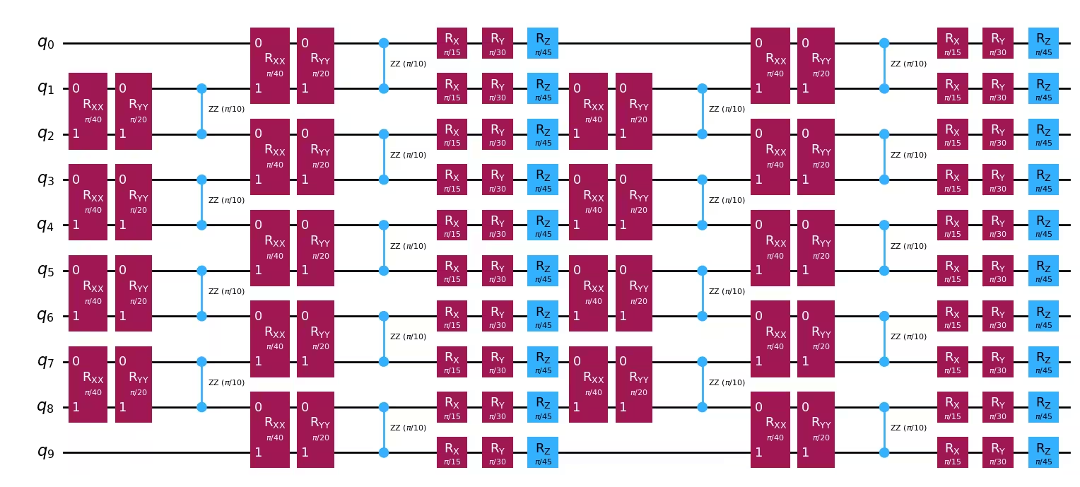
From the qubit operator, we can generate a quantum circuit which models its time evolution. We have used generate_time_evolution_circuit with Lie Trotter decomposition to construct the time evolution circuit.

circuit = generate_time_evolution_circuit(
    hamiltonian,
    time=0.2,
    synthesis=LieTrotter(reps=2),
)
circuit.draw("mpl", style="iqp", fold=-1)

Output:

Step 2: Optimize problem for quantum hardware execution

Create circuit slices to backpropagate

The backpropagate function backpropagates entire circuit slices at a time. Therefore, the choice of slicing can have an impact on how well backpropagation performs for a given problem. Here, we will group gates of the same type into slices using the slice_by_depth function.

For a more detailed discussion on circuit slicing, check out this how-to guide of the qiskit-addon-utils package.

slices = slice_by_depth(circuit, max_slice_depth=1)
print(f"Separated the circuit into {len(slices)} slices.")

Output:

Separated the circuit into 18 slices.

Constrain how large the operator can grow during backpropagation

During backpropagation, the number of terms in the operator will generally approach $2^L$ quickly, where $L$ is the number of slices. When two terms in the operator do not commute qubit-wise, we need separate circuits to obtain the expectation values corresponding to them. For example, if we have a two-qubit observable $O = 0.1 XX + 0.3 IZ - 0.5 IX$, then since $[XX,IX] = 0$, measurement in a single basis is sufficient to calculate the expectation values for these two terms. However, $IZ$ anti-commutes with the other two terms, so we need a separate basis measurement to calculate the expectation value of $IZ$. In other words, we need two circuits instead of one to calculate $\langle O \rangle$. As the number of terms in the operator increases, there is a possibility that the required number of circuit executions also increases.

The size of the operator can be bounded by specifying the operator_budget kwarg of the backpropagate function, which accepts an OperatorBudget instance.

To control the amount of extra resources (number of circuit execution, and hence the QPU time required) allocated, we restrict the maximum number of qubit-wise commuting Pauli groups that the backpropagated observable is allowed to have. Here we specify that backpropagation should stop when the number of qubit-wise commuting Pauli groups in the operator grows past eight.

op_budget = OperatorBudget(max_qwc_groups=8)

Backpropagate slices from the circuit

First we specify the observable to be $M_Z = \frac{1}{N} \sum_{i=1}^N \langle Z_i \rangle$, $N$ being the number of qubits. We will backpropagate slices from the time-evolution circuit until the terms in the observable can no longer be combined into eight or fewer qubit-wise commuting Pauli groups.

observable = SparsePauliOp.from_sparse_list(
    [("Z", [i], 1 / num_qubits) for i in range(num_qubits)],
    num_qubits=num_qubits,
)
observable

Output:

SparsePauliOp(['IIIIIIIIIZ', 'IIIIIIIIZI', 'IIIIIIIZII', 'IIIIIIZIII', 'IIIIIZIIII', 'IIIIZIIIII', 'IIIZIIIIII', 'IIZIIIIIII', 'IZIIIIIIII', 'ZIIIIIIIII'],
              coeffs=[0.1+0.j, 0.1+0.j, 0.1+0.j, 0.1+0.j, 0.1+0.j, 0.1+0.j, 0.1+0.j, 0.1+0.j,
 0.1+0.j, 0.1+0.j])

Below you will see that we backpropagated six slices, and the terms were combined into six and not eight groups. This implies that backpropagating one more slice would cause the number of Pauli groups to exceed eight. We can verify that this is the case by inspecting the returned metadata. Also note that in this portion the circuit transformation is exact. That is, no terms of the new observable $O’$ were truncated. The backpropagated circuit and the backpropagated operator give the exact outcome as the original circuit and operator.

# Backpropagate slices onto the observable
bp_obs, remaining_slices, metadata = backpropagate(
    observable, slices, operator_budget=op_budget
)
# Recombine the slices remaining after backpropagation
bp_circuit = combine_slices(remaining_slices)

print(f"Backpropagated {metadata.num_backpropagated_slices} slices.")
print(
    f"New observable has {len(bp_obs.paulis)} terms, which can be combined into {len(bp_obs.group_commuting(qubit_wise=True))} groups."
)
print(
    f"Note that backpropagating one more slice would result in {metadata.backpropagation_history[-1].num_paulis[0]} terms "
    f"across {metadata.backpropagation_history[-1].num_qwc_groups} groups."
)
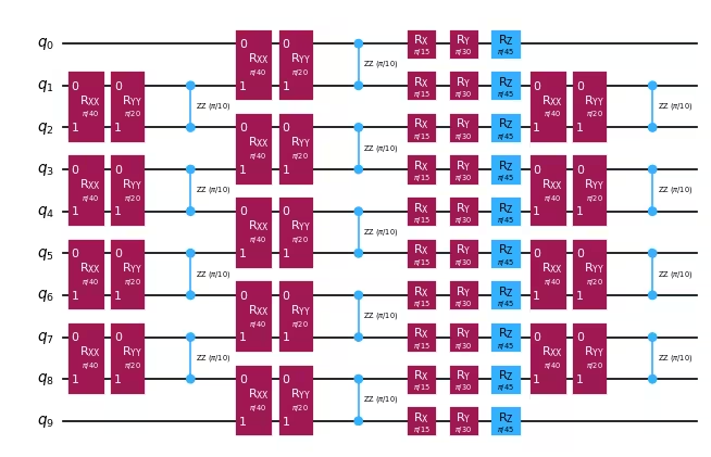
print("The remaining circuit after backpropagation looks as follows:")
bp_circuit.draw("mpl", fold=-1, scale=0.6)

Output:

Backpropagated 6 slices.
New observable has 60 terms, which can be combined into 6 groups.
Note that backpropagating one more slice would result in 114 terms across 12 groups.
The remaining circuit after backpropagation looks as follows:

For the small-scale example on a simulator, we will not use truncation. This is because in the absence of noise, the circuit with and without backpropagation leads to the same result, and truncation makes the result worse due to the added approximation.

Transpile the circuits into the basis gate set

Now we transpile both the original and the backpropagated circuits into the basis gate of the backend. We don't need to transpile on the actual backend since we are going to run on a simulator for the small instance.

service = QiskitRuntimeService()
backend = service.least_busy(
    operational=True, simulator=False, min_num_qubits=133
)
print(backend)

Output:

<IBMBackend('ibm_kingston')>

pm_basis = generate_preset_pass_manager(
    optimization_level=3, basis_gates=backend.configuration().basis_gates
)
isa_circuit = pm_basis.run(circuit)
isa_bp_circuit = pm_basis.run(bp_circuit)

Step 3: Execute using Qiskit primitives

First, we create two Primitive Unified Blocs (PUBs) corresponding to the original circuit, and the backpropagated circuit. Then we execute the pubs on an ideal Estimator to obtain the expectation values.

pubs = [(isa_circuit, observable), (isa_bp_circuit, bp_obs)]

rng = np.random.default_rng()
estimator = StatevectorEstimator(seed=rng)
job = estimator.run(pubs)

Step 4: Post-process and return result in desired classical format

Now we obtain the expectation values of the original and backpropagated circuits.

primitive_result = job.result()
circuit_expval = primitive_result[0].data.evs.item()
bp_circuit_expval = primitive_result[1].data.evs.item()

methods = [
    "No backpropagation",
    "Backpropagation",
]
values = [circuit_expval, bp_circuit_expval]

ax = plt.gca()
plt.bar(methods, values, color="#a56eff", width=0.4, edgecolor="#8a3ffc")
ax.set_ylim([0.6, 0.92])
ax.set_ylabel(r"$M_Z$", fontsize=12)

Output:

Text(0, 0.5, '$M_Z$')

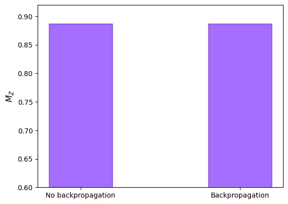
As expected, the two expectation values agree. Because we are running on a noiseless statevector simulator, backpropagation is an exact transformation of the circuit-observable pair, so the original and backpropagated workflows must produce the same value of $M_Z$. The benefit of backpropagation only becomes apparent on noisy hardware, where the shorter backpropagated circuit accumulates less error, as illustrated in the large-scale hardware example below.

Large-scale hardware example

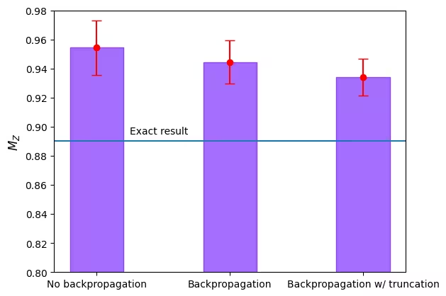
When developing an experiment, it's useful to start with a small circuit to make visualizations and simulations easier. Now we look into operator backpropagation for a 50-qubit Heisenberg Hamiltonian with the same set of values for the $J$ and $h$ parameters and the same observable $M_Z$, but for four Trotter steps. The ideal expectation value at this scale cannot be calculated in a brute force method, so we use a tensor network and obtain the ideal expectation value to be $\simeq 0.89$.

Along with backpropagation, in this large-scale example, we also introduce backpropagation with truncation. Ideally we want to backpropagate as much as possible to reduce the depth of the effective circuit. However, it often leads to a large number of non-commuting terms in the updated observable, increasing the quantum overhead. Therefore, we can eliminate observable terms with small coefficients using a practice called truncation. While truncation allows more propagation by reducing the number of terms in the updated observable, it also introduces some approximation. Therefore, it is necessary to restrict the truncation within some limits so that the approximation error does not overwhelm the reduction in noise obtained from deeper backpropagation.

To restrict the amount of truncation, we allot an error budget for each slice as well as the total error budget over the entire backpropagated circuit using the setup_budget function. This ensures that the truncation is controlled for each slice as well as for the entire circuit. See also this guide for other ways of allocating the budget.

num_qubits = 50
layout = [(i - 1, i) for i in range(1, num_qubits)]

# Instantiate a CouplingMap object
coupling_map = CouplingMap(layout)

hamiltonian = generate_xyz_hamiltonian(
    coupling_map,
    coupling_constants=(np.pi / 8, np.pi / 4, np.pi / 2),
    ext_magnetic_field=(np.pi / 3, np.pi / 6, np.pi / 9),
)

# Generate a time evolution circuit for the Hamiltonian
circuit = generate_time_evolution_circuit(
    hamiltonian,
    time=0.2,
    synthesis=LieTrotter(reps=4),
)

# Define the observable to measure
observable = SparsePauliOp.from_sparse_list(
    [("Z", [i], 1 / num_qubits) for i in range(num_qubits)],
    num_qubits,
)

slices = slice_by_depth(circuit, max_slice_depth=1)

# Define the maximum number of qwc groups allowed in the backpropagated observable, and the truncation error budget
op_budget = OperatorBudget(max_qwc_groups=15)
truncation_error_budget = setup_budget(
    max_error_total=0.03, max_error_per_slice=0.005
)

# First backpropagation without truncation
bp_obs, remaining_slices, metadata = backpropagate(
    observable, slices, operator_budget=op_budget
)
bp_circuit = combine_slices(remaining_slices)

# Now backpropagate with truncation, using the same operator budget and the defined truncation error budget
bp_obs_trunc, remaining_slices_trunc, metadata = backpropagate(
    observable,
    slices,
    operator_budget=op_budget,
    truncation_error_budget=truncation_error_budget,
)
bp_circuit_trunc = combine_slices(
    remaining_slices_trunc, include_barriers=False
)

# Now we transpile the original circuit and the two backpropagated circuits, and apply the layout to the corresponding observables
pm = generate_preset_pass_manager(optimization_level=3, backend=backend)

isa_circuit = pm.run(circuit)
isa_bp_circuit = pm.run(bp_circuit)
isa_bp_circuit_trunc = pm.run(bp_circuit_trunc)

isa_observable = observable.apply_layout(isa_circuit.layout)
isa_bp_observable = bp_obs.apply_layout(isa_bp_circuit.layout)
isa_bp_observable_trunc = bp_obs_trunc.apply_layout(
    isa_bp_circuit_trunc.layout
)

# Compare the 2-qubit depth of each transpiled circuit to see how much depth backpropagation saved
print(
    f"2-qubit depth without backpropagation: {isa_circuit.depth(lambda x: x.operation.num_qubits == 2)}"
)
print(
    f"2-qubit depth with backpropagation: {isa_bp_circuit.depth(lambda x: x.operation.num_qubits == 2)}"
)
print(
    f"2-qubit depth with backpropagation and truncation: {isa_bp_circuit_trunc.depth(lambda x: x.operation.num_qubits == 2)}"
)

pubs = [
    (isa_circuit, isa_observable),
    (isa_bp_circuit, isa_bp_observable),
    (isa_bp_circuit_trunc, isa_bp_observable_trunc),
]

# Now we instantiate the Estimator primitive for the hardware with ZNE and measurement error mitigation
# and compute the three circuits and observables
options = EstimatorOptions()
options.default_precision = 0.01
options.resilience_level = 2
options.resilience.zne.noise_factors = [1, 1.2, 1.4]
options.resilience.zne.extrapolator = ["linear"]
estimator = EstimatorV2(mode=backend, options=options)

estimator.options.environment.job_tags = ["TUT_OBP"]
job = estimator.run(pubs)

# Retrieve the results and the standard deviations
result_no_bp = job.result()[0].data.evs.item()
result_bp = job.result()[1].data.evs.item()
result_bp_trunc = job.result()[2].data.evs.item()

std_no_bp = job.result()[0].data.stds.item()
std_bp = job.result()[1].data.stds.item()
std_bp_trunc = job.result()[2].data.stds.item()

Output:

2-qubit depth without backpropagation: 24
2-qubit depth with backpropagation: 20
2-qubit depth with backpropagation and truncation: 18

print(f"Expectation value without backpropagation: {result_no_bp}")
print(f"Backpropagated expectation value: {result_bp}")
print(f"Backpropagated expectation value with truncation: {result_bp_trunc}")

Output:

Expectation value without backpropagation: 0.9543907942381811
Backpropagated expectation value: 0.9445337385406468
Backpropagated expectation value with truncation: 0.934050286970965

# Plot the results
methods = [
    "No backpropagation",
    "Backpropagation",
    "Backpropagation w/ truncation",
]
values = [result_no_bp, result_bp, result_bp_trunc]
error_bars = [std_no_bp, std_bp, std_bp_trunc]

ax = plt.gca()
plt.bar(methods, values, color="#a56eff", width=0.4, edgecolor="#8a3ffc")
plt.errorbar(methods, values, yerr=error_bars, fmt="o", color="r", capsize=5)
plt.axhline(0.89)
ax.set_ylim([0.8, 0.98])
plt.text(0.25, 0.895, "Exact result")
ax.set_ylabel(r"$M_Z$", fontsize=12)

Output:

Text(0, 0.5, '$M_Z$')

Next steps

If you found this work interesting, you might be interested in the following material: