Multi-product formulas to reduce Trotter error

Usage estimate: Four minutes on a Heron r2 processor (NOTE: This is an estimate only. Your runtime may vary.)

Learning outcomes

After completing this tutorial, you can expect to understand the following information:

• How multi-product formulas (MPFs) reduce Trotter error in Hamiltonian simulation by combining expectation values from multiple shallow circuits
• When MPFs are beneficial over standard product formulas and when they are not the right tool
• How to compute static and dynamic MPF coefficients using the qiskit_addon_mpf package
• How to execute an MPF workflow end-to-end on IBM Quantum® hardware, including transpilation, error mitigation, and post-processing

Prerequisites

We suggest that users are familiar with the following topics before going through this tutorial:

• Compilation methods for Hamiltonian simulation circuits — introduces Trotter (product formula) circuits in Qiskit.
• Product formulas in Qiskit, in particular the SuzukiTrotter and LieTrotter synthesis classes.
• Qiskit primitives and the Estimator interface.

Background

What are multi-product formulas?

When simulating quantum systems on a quantum computer, a central task is to approximate the time-evolution operator $e^{-iHt}$ for a Hamiltonian $H$. The standard approach uses product formulas (PFs), also known as Trotter-Suzuki decompositions. These decompose $H = \sum_{a=1}^d F_a$ into terms whose individual unitaries $e^{-iF_a t}$ are efficient to implement, and then approximate the full evolution as an ordered product of these simpler unitaries.

The first-order product formula (Lie-Trotter) is:

which incurs a quadratic error: $S_1(t) = e^{-iHt} + \mathcal{O}(t^2)$. Higher-order symmetric formulas $S_{2\chi}(t)$, where $\chi$ labels the order of the symmetric product formula (see Ref. [1]), converge faster as $e^{-iHt} + \mathcal{O}(t^{2\chi+1})$, but at the cost of deeper circuits per step.

To reduce the error at a fixed order $\chi$, one usually splits the total evolution time $t$ into $k$ smaller Trotter steps. Each step approximates $e^{-iHt/k}$ by a product formula and the steps are concatenated:

For a $2\chi$-order symmetric formula the residual Trotter error then scales as $\mathcal{O}\!\left(t^{2\chi+1} / k^{2\chi}\right)$. So increasing $k$ rapidly suppresses the Trotter error — but it also linearly deepens the circuit, and on noisy hardware that means more accumulated gate noise. This tension between Trotter error (favors larger $k$) and hardware noise (favors smaller $k$) is precisely what multi-product formulas are designed to resolve. Note that MPFs are about combining results from different choices of $k$ at a fixed order $\chi$ — they do not change the order of the underlying product formula.

Multi-product formulas (MPFs) [1] construct a weighted linear combination of expectation values obtained from several shallower Trotter circuits, each using a different number of Trotter steps $k_1, k_2, \ldots, k_r$ (a set of $r$ step counts):

where $\langle A \rangle_{k_j}(t)$ is the expectation value of an observable $A$ at time $t$ estimated from a Trotter circuit with $k_j$ steps, and the coefficients $\{x_j\}_{j=1}^r$ are chosen so that the leading Trotter-error terms in the combination cancel. We will revisit this expression in Step 4, where we evaluate it explicitly to combine our Trotter results. The key practical point is that the deepest circuit in the MPF only needs $k_{\max}$ steps, which is much smaller than the single $k$ that would be required to reach the same effective Trotter error directly. The shallower circuits make the MPF approach better suited to noisy hardware.

How are the coefficients determined?

There are two families of MPF coefficients:

Static coefficients are independent of the Hamiltonian, the initial state, and the evolution time. They are found by solving a linear system $Ax = b$ that enforces cancellation of the leading Trotter error terms. For a set of Trotter steps $\{k_j\}_{j=1}^r$ used with a $2\chi$-order symmetric product formula, expanding the Trotter error in inverse powers of $k_j$ leads to constraint equations of the form:

where the integer exponents $\{\eta_n\}$ are the orders of the successive Trotter-error terms for the chosen product formula. For a symmetric $2\chi$-order PF, the leading error in $\left[S_{2\chi}(t/k)\right]^k$ scales as $1/k^{2\chi}$, with subsequent corrections at $1/k^{2\chi+2}, 1/k^{2\chi+4}, \ldots$ — so the exponents are $\eta_n = 2\chi + 2n$. For non-symmetric PFs, both odd and even powers contribute and $\eta_n = 2\chi + n$. See Ref. [1] for the full derivation. The first equation in the system above ensures unbiasedness (the MPF reproduces the exact expectation value in the $k_j \to \infty$ limit), and the remaining $r-1$ equations successively cancel the first $r-1$ Trotter-error terms. When the resulting $L_1$-norm $\|x\|_1$ is too large (which amplifies sampling noise), you can instead solve an approximate optimization that caps $\|x\|_1$ while minimizing $\|Ax - b\|$.

Dynamic coefficients [2], [3] additionally depend on the Hamiltonian, initial state, and evolution time $t$. They minimize the Frobenius-norm distance between the true time-evolved state and the MPF approximation:

where $M_{ij}(t) = \mathrm{Tr}[\rho_{k_i}(t)\,\rho_{k_j}(t)]$ is the Gram matrix of overlaps between Trotter-evolved states for different step counts $k_i, k_j$, and $L_i(t) = \mathrm{Tr}[\rho(t)\,\rho_{k_i}(t)]$ measures overlap with the (approximate) exact state. In this tutorial these quantities are computed efficiently using tensor-network methods, specifically the TeNPy-based backends in qiskit_addon_mpf.

When to use MPFs

MPFs are most beneficial when:

• Circuit depth is the bottleneck. If hardware noise limits the depth you can run, use MPFs to achieve higher effective Trotter accuracy from shallower circuits.
• You need accurate expectation values, not full state preparation. MPFs operate at the level of expectation values — they combine classical numbers, not quantum states. They are therefore ideal for observable estimation when using the Estimator primitive.
• You combine a modest number of Trotter-step counts. Typically combining $r = 3$–$5$ different step counts $k_j$ is sufficient to cancel several leading Trotter-error terms while keeping $\|x\|_1$ manageable.

When MPFs might not help

• Very short evolution times. When $t$ is small enough that a single low-order Trotter formula is already accurate, the overhead of running multiple circuits is unnecessary.
• State-preparation tasks. MPFs produce a corrected expectation value, not a corrected quantum state. If you need the actual time-evolved state (for example, as input to another quantum subroutine), MPFs do not apply.
• Trotter-step counts that violate the convergence regime. The static-coefficient derivation expands each individual $\left[S_{2\chi}(t/k_j)\right]^{k_j}$ as a series in $t/k_j$; this expansion only converges well when $t/k_{\min} \lesssim 1$. If $k_{\min}$ is chosen too small for the given $t$, the shallowest circuit is far outside the perturbative regime, the higher-order error terms that the MPF leaves uncanceled become large, and the cancellation can require large coefficients. The $L_1$-norm $\|x\|_1$ is the practical diagnostic: when $\|x\|_1 \gg 1$, the sampling overhead $\propto \|x\|_1^2$ might outweigh the Trotter-error reduction. See the guide on choosing Trotter steps for details.

What this tutorial covers

This tutorial walks through an end-to-end MPF workflow in two stages. First, a small-scale simulator example (10-qubit Heisenberg chain) demonstrates how to set up the problem, compute static and dynamic MPF coefficients, and compare the resulting expectation values against exact diagonalization. Then, a large-scale hardware example (50-qubit XXZ chain) shows how to transpile, execute on IBM Quantum hardware with error mitigation, and post-process results using the MPF coefficients. Throughout, we use the qiskit_addon_mpf package alongside standard Qiskit tools.

Requirements

Before starting this tutorial, ensure that you have the following installed:

• Qiskit SDK v2.0 or later, with visualization support
• Qiskit Runtime v0.22 or later (pip install qiskit-ibm-runtime)
• Qiskit Aer simulator (pip install qiskit-aer)
• MPF Qiskit addon with the TeNPy backend (pip install "qiskit-addon-mpf[tenpy]")
• Qiskit addon utilities (pip install qiskit-addon-utils)
• SciPy (pip install scipy)

Setup

Below we collect all the package imports used throughout this tutorial in a single cell. We also define a CollectAndCollapse transpiler pass that fuses adjacent rxx and ryy rotations into a single XXPlusYYGate. This pass is applied both during circuit construction in Step 1 (to keep the gate count low) and indirectly when we extract the layered structure for the dynamic MPF in Step 4 (TeNPy expects two-qubit gates, not pairs of unfused rotations).

import warnings

import numpy as np
import matplotlib.pyplot as plt
from functools import partial
from copy import deepcopy

from qiskit import QuantumCircuit
from qiskit.quantum_info import Pauli, SparsePauliOp, Statevector
from qiskit.synthesis import SuzukiTrotter
from qiskit.transpiler import CouplingMap, PassManager
from qiskit.transpiler.preset_passmanagers import generate_preset_pass_manager
from qiskit.circuit.library import XXPlusYYGate
from qiskit.transpiler.passes.optimization.collect_and_collapse import (
    CollectAndCollapse,
    collect_using_filter_function,
    collapse_to_operation,
)

from qiskit_aer import AerSimulator
from qiskit_ibm_runtime import EstimatorV2 as Estimator, QiskitRuntimeService

from qiskit_addon_utils.problem_generators import (
    generate_xyz_hamiltonian,
    generate_time_evolution_circuit,
)
from qiskit_addon_utils.slicing import slice_by_depth
from qiskit_addon_mpf.static import setup_static_lse
from qiskit_addon_mpf.dynamic import setup_dynamic_lse
from qiskit_addon_mpf.costs import (
    setup_exact_problem,
    setup_sum_of_squares_problem,
    setup_frobenius_problem,
)
from qiskit_addon_mpf.backends.tenpy_layers import (
    LayerModel,
    LayerwiseEvolver,
)
from qiskit_addon_mpf.backends.tenpy_tebd import MPOState, MPS_neel_state

from scipy.linalg import expm

# Suppress TeNPy's `unit_cell_width` future-API warning. The default
# (`unit_cell_width=len(sites)`) is correct for Chain lattices, which is what
# `CouplingMap.from_line(...)` produces here, so the warning is informational.
warnings.filterwarnings(
    "ignore",
    message=r".*unit_cell_width.*",
    category=UserWarning,
)


# --- Helper: collect XX + YY rotations into a single gate ---
def filter_function(node):
    return node.op.name in {"rxx", "ryy"}


collect_function = partial(
    collect_using_filter_function,
    filter_function=filter_function,
    split_blocks=True,
    min_block_size=1,
)


def collapse_to_xx_plus_yy(block):
    param = 0.0
    for node in block.data:
        param += node.operation.params[0]
    return XXPlusYYGate(param)


collapse_function = partial(
    collapse_to_operation,
    collapse_function=collapse_to_xx_plus_yy,
)

pm = PassManager()
pm.append(CollectAndCollapse(collect_function, collapse_function))

Small-scale simulator example

Step 1: Map classical inputs to a quantum problem

We begin with a 10-qubit Heisenberg model on a line, using the Néel state $\vert 0101\ldots01 \rangle$ as the initial state. The Hamiltonian is:

where $J$ is the nearest-neighbor coupling strength. We measure the ZZ correlator $Z_{L/2-1} Z_{L/2}$ on a pair of qubits in the middle of the chain, and use Trotter steps $k_j = [1, 2, 4]$ with a second-order product formula.

L = 10

# Generate coupling map and Hamiltonian
coupling_map = CouplingMap.from_line(L, bidirectional=False)

hamiltonian = generate_xyz_hamiltonian(
    coupling_map,
    coupling_constants=(1.0, 1.0, 1.0),
    ext_magnetic_field=(0.0, 0.0, 0.0),
)
print(hamiltonian)

Output:

SparsePauliOp(['IIIIIIIXXI', 'IIIIIIIYYI', 'IIIIIIIZZI', 'IIIIIXXIII', 'IIIIIYYIII', 'IIIIIZZIII', 'IIIXXIIIII', 'IIIYYIIIII', 'IIIZZIIIII', 'IXXIIIIIII', 'IYYIIIIIII', 'IZZIIIIIII', 'IIIIIIIIXX', 'IIIIIIIIYY', 'IIIIIIIIZZ', 'IIIIIIXXII', 'IIIIIIYYII', 'IIIIIIZZII', 'IIIIXXIIII', 'IIIIYYIIII', 'IIIIZZIIII', 'IIXXIIIIII', 'IIYYIIIIII', 'IIZZIIIIII', 'XXIIIIIIII', 'YYIIIIIIII', 'ZZIIIIIIII'],
              coeffs=[1.+0.j, 1.+0.j, 1.+0.j, 1.+0.j, 1.+0.j, 1.+0.j, 1.+0.j, 1.+0.j, 1.+0.j,
 1.+0.j, 1.+0.j, 1.+0.j, 1.+0.j, 1.+0.j, 1.+0.j, 1.+0.j, 1.+0.j, 1.+0.j,
 1.+0.j, 1.+0.j, 1.+0.j, 1.+0.j, 1.+0.j, 1.+0.j, 1.+0.j, 1.+0.j, 1.+0.j])

# Observable: ZZ on the middle pair of qubits
observable = SparsePauliOp.from_sparse_list(
    [("ZZ", (L // 2 - 1, L // 2), 1.0)], num_qubits=L
)
print(observable)

Output:

SparsePauliOp(['IIIIZZIIII'],
              coeffs=[1.+0.j])

# MPF parameters
mpf_trotter_steps = [1, 2, 4]
order = 2
symmetric = False

trotter_times = np.arange(0.5, 1.55, 0.1)
exact_evolution_times = np.arange(trotter_times[0], 1.55, 0.05)

Build Trotter circuits

We create the circuits implementing the approximate Trotter time-evolutions for each time point and each Trotter step count. The CollectAndCollapse pass defined in the Setup section collects XX and YY rotations into single XX+YY gates, to prepare for more efficient tensor-network simulation later.

# Initial Neel state preparation
initial_state_circ = QuantumCircuit(L)
initial_state_circ.x([i for i in range(L) if i % 2 != 0])


all_circs = []
for total_time in trotter_times:
    mpf_trotter_circs = [
        generate_time_evolution_circuit(
            hamiltonian,
            time=total_time,
            synthesis=SuzukiTrotter(reps=num_steps, order=order),
        )
        for num_steps in mpf_trotter_steps
    ]

    mpf_trotter_circs = pm.run(
        mpf_trotter_circs
    )  # Collect XX and YY into XX + YY

    mpf_circuits = [
        initial_state_circ.compose(circuit) for circuit in mpf_trotter_circs
    ]
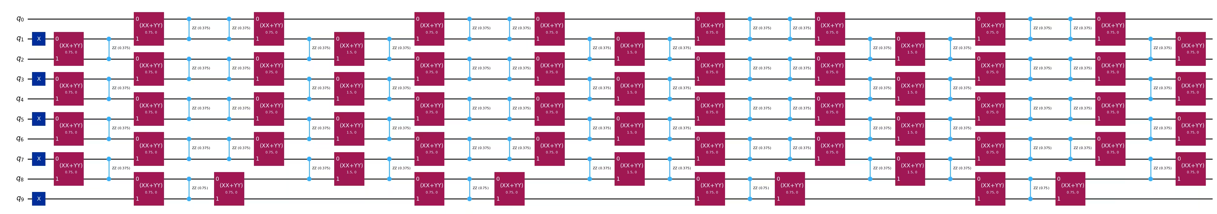
    all_circs.append(mpf_circuits)

mpf_circuits[-1].draw("mpl", fold=-1)

Output:

Step 2: Optimize problem for quantum hardware execution

For the small-scale example we target the Aer simulator. Two transformations happen before the circuits are ready to execute:

1. Gate collection at the Hamiltonian-simulation level. In the Setup cell we built a CollectAndCollapse pass that fuses adjacent rxx and ryy rotations into a single XXPlusYYGate. We already applied this pass when we built the Trotter circuits in Step 1 (the pm.run(...) call). This both reduces the two-qubit gate count and produces a structure that is more amenable to tensor-network simulation for the dynamic-coefficient computation later.

2. Lowering to the simulator's ISA. Below we run the Qiskit preset pass manager at optimization_level=3 to lower each Trotter circuit to the simulator's instruction-set architecture (ISA).

aer_sim = AerSimulator()
pm_sim = generate_preset_pass_manager(backend=aer_sim, optimization_level=3)

isa_circs_all_times = [
    pm_sim.run([deepcopy(c) for c in mpf_circuits])
    for mpf_circuits in all_circs
]

Step 3: Execute using Qiskit primitives

For the small-scale example we run the ISA-lowered Trotter circuits through the EstimatorV2 primitive backed by Aer. Doing so gives us a noiseless reference value for each $(k_j, t)$ pair — these are the $\langle A \rangle_{k_j}(t)$ values that the MPF will combine in Step 4. We sweep over evolution times so that we can later plot the full time-series curve of each individual product formula and of the MPF.

estimator = Estimator(mode=aer_sim)

mpf_expvals_all_times, mpf_stds_all_times = [], []
for isa_circuits in isa_circs_all_times:
    result = estimator.run(
        [(circuit, observable) for circuit in isa_circuits], precision=0.005
    ).result()
    mpf_expvals_all_times.append([res.data.evs for res in result])
    mpf_stds_all_times.append([res.data.stds for res in result])

Step 4: Post-process and return result in desired classical format

Step 4 is where the MPF is actually constructed. Even though the coefficients $x_j$ are computed here (and, for the dynamic variant, this computation can be intensive), conceptually they are a classical recipe for combining the quantum measurements from Step 3 into a single corrected expectation value — so we treat the whole coefficient and combination workflow as post-processing.

To assess how well the MPF tracks the true dynamics, we first compute the exact time-evolved expectation values by directly exponentiating the Hamiltonian. This is only tractable because $L = 10$; in the large-scale hardware example below we will have to rely on tensor-network estimates instead.

exact_expvals = []
for t in exact_evolution_times:
    exp_H = expm(-1j * t * hamiltonian.to_matrix())
    initial_state = Statevector(initial_state_circ).data
    time_evolved_state = exp_H @ initial_state

    exact_obs = (
        time_evolved_state.conj()
        @ observable.to_matrix()
        @ time_evolved_state
    ).real
    exact_expvals.append(exact_obs)

Static MPF coefficients

Static MPFs use coefficients $x_j$ that are independent of the evolution time, the Hamiltonian, and the initial state. We set up the linear system $Ax = b$ described in the Background and solve for the coefficients. The matrix $A$ is determined by the Trotter step counts $k_j$, the order $\chi$ of the product formula, and whether the formula is symmetric (which controls the exponents $\eta_n$).

For our small-scale example we use $k_j = [1, 2, 4]$ with a non-symmetric order-$2\chi=2$ Suzuki-Trotter formula (so $\chi=1$ and $\eta_n = 2 + n$, giving $\eta_0 = 2,\, \eta_1 = 3$). The system becomes:

The first row enforces unbiasedness ($\sum_j x_j = 1$); the second and third rows cancel the leading $1/k^2$ and next-order $1/k^3$ Trotter-error terms, respectively.

Set up the LSE

We use setup_static_lse from qiskit_addon_mpf.static to assemble the matrix $A$ and right-hand-side vector $b$ described above. The matrix $A$ depends not only on $k_j$ but also on our choice of product formula — in particular its order $\chi$ and whether it is symmetric. The symmetric flag controls the exponent pattern $\eta_n$ (symmetric formulas only produce even-power Trotter-error terms; see Ref. [1]). Note that, as shown in Ref. [2], setting symmetric=True is not strictly necessary even when the underlying PF is symmetric — the non-symmetric LSE remains valid (it enforces extra unneeded constraints).

For our example we have already set order = 2 and symmetric = False in Step 1.

lse = setup_static_lse(mpf_trotter_steps, order=order, symmetric=symmetric)

Inspect the constructed matrix $A$ and vector $b$ to confirm they match the system written above.

lse.A

Output:

array([[1.      , 1.      , 1.      ],
       [1.      , 0.25    , 0.0625  ],
       [1.      , 0.125   , 0.015625]])

lse.b

Output:

array([1., 0., 0.])

With the LSE in hand, we solve for the static coefficients $x_j$ via lse.solve() (this is the direct $x = A^{-1}b$ solution).

mpf_coeffs = lse.solve()
print(
    f"The static coefficients associated with the ansatze are: {mpf_coeffs}"
)

Output:

The static coefficients associated with the ansatze are: [ 0.04761905 -0.57142857  1.52380952]

Optimize for $x$ using an exact model

Alternatively to computing $x = A^{-1}b$, you can use setup_exact_model to construct a cvxpy.Problem instance that uses the LSE as constraints and whose optimal solution will yield $x$.

model_exact, coeffs_exact = setup_exact_problem(lse)
model_exact.solve()
print(coeffs_exact.value)

Output:

[ 0.04761905 -0.57142857  1.52380952]

print(
    "L1 norm of the exact coefficients:",
    np.linalg.norm(coeffs_exact.value, ord=1),
)

Output:

L1 norm of the exact coefficients: 2.1428571428556378

Optimize for $x$ using an approximate model

It might happen that the $L_1$ norm for the chosen set of $k_j$ values is deemed too high. If that is the case and you cannot choose a different set of $k_j$ values, you can use an approximate solution that constrains the $L_1$-norm to a chosen threshold while minimizing $\|Ax - b\|$. Check out the guide on How to use the approximate model.

model_approx, coeffs_approx = setup_sum_of_squares_problem(
    lse, max_l1_norm=1.5
)
model_approx.solve()
print(coeffs_approx.value)
print(
    "L1 norm of the approximate coefficients:",
    np.linalg.norm(coeffs_approx.value, ord=1),
)

Output:

[-1.10294118e-03 -2.48897059e-01  1.25000000e+00]
L1 norm of the approximate coefficients: 1.5

Dynamic MPF coefficients

The static MPF cancels Trotter-error terms in a Hamiltonian- and state-agnostic way, so it does not necessarily produce the smallest possible approximation error for a given Hamiltonian and initial state. The dynamic MPF (Refs. [2], [3]) instead finds time-dependent coefficients $x_i(t)$ that minimize the Frobenius-norm distance $\|\rho(t) - \mu^D(t)\|_F^2$ at each time $t$. As shown in the Background, this requires the overlap matrix $M_{ij}(t)$ between Trotter-evolved states and the overlap $L_i(t)$ with the exact state — both of which we estimate using tensor-network (TeNPy) backends in qiskit_addon_mpf.

To set up the dynamic LSE we need three ingredients:

1. An approximate evolver factory that the addon will run for each $k_j$ to produce $\rho_{k_j}(t)$ as an MPS/MPO. We build it from the layered structure of the order-$2$ Trotter circuit (one layer per slice_by_depth), wrapped as a LayerwiseEvolver with TeNPy truncation parameters.
2. An exact evolver factory that produces a high-accuracy reference $\rho(t)$. We use a small-time-step fourth-order Suzuki-Trotter circuit (dt=0.1, order=4) as a proxy for exact evolution.
3. An identity factory and an initial-state MPS that seed the TeNPy simulation.

The cell below constructs the approximate evolver factory.

# Create approximate time-evolution circuits
single_2nd_order_circ = generate_time_evolution_circuit(
    hamiltonian, time=1.0, synthesis=SuzukiTrotter(reps=1, order=order)
)
single_2nd_order_circ = pm.run(single_2nd_order_circ)  # collect XX and YY

# Find layers in the circuit
layers = slice_by_depth(single_2nd_order_circ, max_slice_depth=1)

# Create tensor network models
models = [
    LayerModel.from_quantum_circuit(layer, conserve="Sz") for layer in layers
]

# Create the time-evolution object
approx_factory = partial(
    LayerwiseEvolver,
    layers=models,
    options={
        "preserve_norm": False,
        "trunc_params": {
            "chi_max": 64,
            "svd_min": 1e-8,
            "trunc_cut": None,
        },
        "max_delta_t": 2,
    },
)

We approximate the exact time-evolved state with a fourth-order Suzuki-Trotter formula using a small time step dt=0.1. The TeNPy truncation parameters can affect accuracy, so it is important to explore a range of values.

single_4th_order_circ = generate_time_evolution_circuit(
    hamiltonian, time=1.0, synthesis=SuzukiTrotter(reps=1, order=4)
)
single_4th_order_circ = pm.run(single_4th_order_circ)
exact_model_layers = [
    LayerModel.from_quantum_circuit(layer, conserve="Sz")
    for layer in slice_by_depth(single_4th_order_circ, max_slice_depth=1)
]

exact_factory = partial(
    LayerwiseEvolver,
    layers=exact_model_layers,
    dt=0.1,
    options={
        "preserve_norm": False,
        "trunc_params": {
            "chi_max": 64,
            "svd_min": 1e-8,
            "trunc_cut": None,
        },
        "max_delta_t": 2,
    },
)

Finally, we define an identity_factory that yields the initial MPO state and prepare the Néel initial state as an MPS that matches the lattice used by the layered Trotter model.

def identity_factory():
    return MPOState.initialize_from_lattice(models[0].lat, conserve=True)


mps_initial_state = MPS_neel_state(models[0].lat)

With the factories in place we now compute the dynamic coefficients at each evolution time. For each $t$, setup_dynamic_lse builds the relevant overlap matrices via TeNPy, and setup_frobenius_problem returns a cvxpy.Problem that minimizes the Frobenius-norm cost. The solver returns coefficients $x_j(t)$ tailored to that time; we collect them in mpf_dynamic_coeffs_list. If the solver fails for a given $t$, we fall back to zero coefficients so the loop continues.

mpf_dynamic_coeffs_list = []
for t in trotter_times:
    print(f"Computing dynamic coefficients for time={t}")
    lse = setup_dynamic_lse(
        mpf_trotter_steps,
        t,
        identity_factory,
        exact_factory,
        approx_factory,
        mps_initial_state,
    )
    problem, coeffs = setup_frobenius_problem(lse)
    try:
        problem.solve()
        mpf_dynamic_coeffs_list.append(coeffs.value)
    except Exception as error:
        mpf_dynamic_coeffs_list.append(np.zeros(len(mpf_trotter_steps)))
        print(error, "Calculation Failed for time", t)
    print("")

Output:

Computing dynamic coefficients for time=0.5

Computing dynamic coefficients for time=0.6

Computing dynamic coefficients for time=0.7

Computing dynamic coefficients for time=0.7999999999999999

Computing dynamic coefficients for time=0.8999999999999999

Computing dynamic coefficients for time=0.9999999999999999

Computing dynamic coefficients for time=1.0999999999999999

Computing dynamic coefficients for time=1.1999999999999997

Computing dynamic coefficients for time=1.2999999999999998

Computing dynamic coefficients for time=1.4

Computing dynamic coefficients for time=1.4999999999999998

Combine Trotter expectation values with the MPF coefficients

Now we evaluate $\langle A \rangle_{\text{MPF}}(t) = \sum_j x_j \, \langle A \rangle_{k_j}(t)$ for each set of coefficients (static-exact, static-approximate, and dynamic), propagate the per-circuit standard errors, and plot the resulting time series against the exact-diagonalization curve.

sym = {1: "^", 2: "s", 4: "p"}
# Get expectation values at all times for each Trotter step
for k, step in enumerate(mpf_trotter_steps):
    trotter_curve, trotter_curve_error = [], []
    for trotter_expvals, trotter_stds in zip(
        mpf_expvals_all_times, mpf_stds_all_times
    ):
        trotter_curve.append(trotter_expvals[k])
        trotter_curve_error.append(trotter_stds[k])

    plt.errorbar(
        trotter_times,
        trotter_curve,
        yerr=trotter_curve_error,
        alpha=0.5,
        markersize=4,
        marker=sym[step],
        color="grey",
        label=f"{mpf_trotter_steps[k]} Trotter steps",
    )

# Get expectation values at all times for the static MPF with exact coeffs
exact_mpf_curve, exact_mpf_curve_error = [], []
for trotter_expvals, trotter_stds in zip(
    mpf_expvals_all_times, mpf_stds_all_times
):
    mpf_std = np.sqrt(
        sum(
            [
                (coeff**2) * (std**2)
                for coeff, std in zip(coeffs_exact.value, trotter_stds)
            ]
        )
    )
    exact_mpf_curve_error.append(mpf_std)
    exact_mpf_curve.append(trotter_expvals @ coeffs_exact.value)

plt.errorbar(
    trotter_times,
    exact_mpf_curve,
    yerr=exact_mpf_curve_error,
    markersize=4,
    marker="o",
    label="Static MPF - Exact",
    color="purple",
)


# Get expectation values at all times for the static MPF with approximate coeffs
approx_mpf_curve, approx_mpf_curve_error = [], []
for trotter_expvals, trotter_stds in zip(
    mpf_expvals_all_times, mpf_stds_all_times
):
    mpf_std = np.sqrt(
        sum(
            [
                (coeff**2) * (std**2)
                for coeff, std in zip(coeffs_approx.value, trotter_stds)
            ]
        )
    )
    approx_mpf_curve_error.append(mpf_std)
    approx_mpf_curve.append(trotter_expvals @ coeffs_approx.value)

plt.errorbar(
    trotter_times,
    approx_mpf_curve,
    yerr=approx_mpf_curve_error,
    markersize=4,
    marker="o",
    label="Static MPF - Approx",
    color="orange",
)


# Get expectation values at all times for the dynamic MPF
dynamic_mpf_curve, dynamic_mpf_curve_error = [], []
for trotter_expvals, trotter_stds, dynamic_coeffs in zip(
    mpf_expvals_all_times, mpf_stds_all_times, mpf_dynamic_coeffs_list
):
    mpf_std = np.sqrt(
        sum(
            [
                (coeff**2) * (std**2)
                for coeff, std in zip(dynamic_coeffs, trotter_stds)
            ]
        )
    )
    dynamic_mpf_curve_error.append(mpf_std)
    dynamic_mpf_curve.append(trotter_expvals @ dynamic_coeffs)

plt.errorbar(
    trotter_times,
    dynamic_mpf_curve,
    yerr=dynamic_mpf_curve_error,
    markersize=4,
    marker="o",
    label="Dynamic MPF",
    color="pink",
)


# Exact expectation values
plt.plot(
    exact_evolution_times,
    exact_expvals,
    color="red",
    linestyle="--",
    label="Exact time-evolution",
)

plt.title(f"$\\langle Z_{{{L//2-1}}} Z_{{{L//2}}} \\rangle$ vs time")
plt.xlabel("Time")
plt.ylabel("Expectation Value")
plt.legend(loc="upper center", bbox_to_anchor=(0.5, -0.2), ncol=2)
plt.grid(alpha=0.1)
plt.tight_layout()
plt.show()

Output:

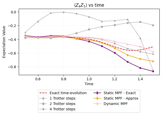
The plot above illustrates the interplay between Trotter error and sampling error.

• Trotter error. The individual product formulas (grey markers) deviate from the exact curve more and more as time grows. The $k=1$ circuit has the largest deviation and is the shallowest, but it is also already in the regime where $t/k \gtrsim 1$, so the leading $1/k^{2}$ error term is large. The MPF combinations (colored markers) cancel several of these leading Trotter-error terms, so they track the exact curve much more closely than any single $k_j$ circuit. The remaining gap reflects the higher-order Trotter terms that the MPF does not cancel: an order-$2$, $r=3$ static MPF only kills the first two error orders, and at large $t/k_{\min}$ the uncanceled tail eventually dominates — so MPF does not guarantee that very shallow circuits remain accurate at arbitrary times.

• Sampling error. The wider error bars on the MPF curves are a direct consequence of the linear combination: propagating independent per-circuit standard errors $\sigma_{k_j}$ gives a total variance $\sigma_{\text{MPF}}^2 = \sum_j x_j^2 \, \sigma_{k_j}^2$. Therefore, the larger the $\|x\|_2$ (and in practice the $\|x\|_1$, which is what we control), the more shots are required to reach a given target uncertainty. This is the trade-off behind the approximate-solver option in the Background: we cap $\|x\|_1$ to keep this overhead manageable. Crucially, unlike Trotter error, sampling error shrinks with $1/\sqrt{N_{\text{shots}}}$, so it can always be reduced by spending more shots.

In the large-scale hardware example below, hardware noise enters as an additional error source on each $\langle A \rangle_{k_j}$, which similarly gets amplified by the MPF coefficients. We will see how error mitigation interacts with MPFs in that section.

Large-scale hardware example

In this section we scale the problem up beyond what is possible to simulate exactly. We reproduce some of the results shown in Ref. [3], using a 50-qubit XXZ chain at time $t = 3$. We follow the same four-step workflow as the small-scale example, now targeting real quantum hardware with error mitigation. As in the template, each step is marked inline in the code, and a single step can span multiple cells when its intermediate outputs are worth inspecting.

The mapping mirrors the small-scale example: define a Hamiltonian, choose Trotter parameters, compute MPF coefficients (static and dynamic), and build circuits. The key differences are:

• An XXZ Hamiltonian on 50 sites with random couplings drawn from $\mathcal{U}(0.5, 1.5)$ (Ref. [3]).
• A symmetric second-order Trotter formula with $k_j = [3, 4, 6]$ (so $\chi=1$, symmetric=True).
• A single fixed evolution time $t = 3$. With $k_{\min}=3$ this gives $t/k_{\min}=1$, keeping the shallow constituents inside the Trotter-convergence regime where the leading-error model the MPF relies on is valid.
• An additional single-circuit comparison run with $k = 10$ Trotter steps, used as a baseline. We chose $k = 10$ because its two-qubit depth on hardware is deeper than the deepest MPF constituent ($k_{\max}=6$) plus the overhead of running multiple MPF circuits — deep enough to be noise-limited, which is the regime in which the MPF combination is expected to outperform the single-circuit baseline. It is a "single deep circuit" comparison against the MPF combination, not a circuit that targets the MPF's effective Trotter error (which would require many more steps).

Note that even though we are still in Step 1 here (mapping and circuit construction), we also pre-compute the dynamic coefficients alongside the static ones in this cell. Dynamic coefficients depend on $H$ and $t$ but not on the quantum measurements, so they can be computed any time before Step 4. We do it now to keep all the MPF-specific setup in one place.

# -------------------------Step 1-------------------------
L = 50
coupling_map = CouplingMap.from_line(L, bidirectional=False)

# XXZ Hamiltonian with random couplings (Ref. [3])
np.random.seed(0)
even_edges = list(coupling_map.get_edges())[::2]
odd_edges = list(coupling_map.get_edges())[1::2]

Js = np.random.uniform(0.5, 1.5, size=L)
hamiltonian = SparsePauliOp(Pauli("I" * L))
for i, edge in enumerate(even_edges + odd_edges):
    hamiltonian += SparsePauliOp.from_sparse_list(
        [
            ("XX", (edge), 2 * Js[i]),
            ("YY", (edge), 2 * Js[i]),
            ("ZZ", (edge), 4 * Js[i]),
        ],
        num_qubits=L,
    )

observable = SparsePauliOp.from_sparse_list(
    [("ZZ", (L // 2 - 1, L // 2), 1.0)], num_qubits=L
)

total_time = 3
mpf_trotter_steps = [3, 4, 6]
order = 2
symmetric = True

# Static coefficients
lse = setup_static_lse(mpf_trotter_steps, order=order, symmetric=symmetric)
mpf_coeffs = lse.solve()
print(f"Static coefficients: {mpf_coeffs}")
print(f"L1 norm: {np.linalg.norm(mpf_coeffs, ord=1)}")

model_approx, coeffs_approx = setup_sum_of_squares_problem(
    lse, max_l1_norm=2.0
)
model_approx.solve()
print(f"Approximate coefficients: {coeffs_approx.value}")
print(f"L1 norm (approx): {np.linalg.norm(coeffs_approx.value, ord=1)}")

# -------------------------Dynamic coefficients-------------------------
single_2nd_order_circ = generate_time_evolution_circuit(
    hamiltonian, time=1.0, synthesis=SuzukiTrotter(reps=1, order=order)
)
single_2nd_order_circ = pm.run(single_2nd_order_circ)

layers = slice_by_depth(single_2nd_order_circ, max_slice_depth=1)
models = [
    LayerModel.from_quantum_circuit(layer, conserve="Sz") for layer in layers
]

approx_factory = partial(
    LayerwiseEvolver,
    layers=models,
    options={
        "preserve_norm": False,
        "trunc_params": {"chi_max": 64, "svd_min": 1e-8, "trunc_cut": None},
        "max_delta_t": 4,
    },
)

single_4th_order_circ = generate_time_evolution_circuit(
    hamiltonian, time=1.0, synthesis=SuzukiTrotter(reps=1, order=4)
)
single_4th_order_circ = pm.run(single_4th_order_circ)
exact_model_layers = [
    LayerModel.from_quantum_circuit(layer, conserve="Sz")
    for layer in slice_by_depth(single_4th_order_circ, max_slice_depth=1)
]

exact_factory = partial(
    LayerwiseEvolver,
    layers=exact_model_layers,
    dt=0.1,
    options={
        "preserve_norm": False,
        "trunc_params": {"chi_max": 64, "svd_min": 1e-8, "trunc_cut": None},
        "max_delta_t": 3,
    },
)


def identity_factory():
    return MPOState.initialize_from_lattice(models[0].lat, conserve=True)


mps_initial_state = MPS_neel_state(models[0].lat)

print(f"Computing dynamic coefficients for time={total_time}")
lse_dyn = setup_dynamic_lse(
    mpf_trotter_steps,
    total_time,
    identity_factory,
    exact_factory,
    approx_factory,
    mps_initial_state,
)
problem, coeffs_dyn = setup_frobenius_problem(lse_dyn)
try:
    problem.solve()
    mpf_dynamic_coeffs = coeffs_dyn.value
except Exception as error:
    mpf_dynamic_coeffs = np.zeros(len(mpf_trotter_steps))
    print(error, "Calculation Failed")

# -------------------------Step 1 (cont): Build circuits-------------------------
mpf_circuits = []
for k in mpf_trotter_steps:
    circuit = QuantumCircuit(L)
    circuit.x([i for i in range(L) if i % 2])
    trotter_circ = generate_time_evolution_circuit(
        hamiltonian,
        synthesis=SuzukiTrotter(reps=k, order=order),
        time=total_time,
    )
    circuit.compose(trotter_circ, qubits=range(L), inplace=True)
    mpf_circuits.append(circuit)

# Baseline "single deep circuit" comparison run with k=10 Trotter steps.
# Its two-qubit depth is deeper than the deepest MPF constituent (k_max=6) plus
# the overhead of running multiple circuits, pushing it into the noise-limited
# regime where MPF is expected to outperform. It does NOT target the MPF's effective
# Trotter error (which would require many more steps).
comp_circuit = QuantumCircuit(L)
comp_circuit.x([i for i in range(L) if i % 2])
trotter_circ = generate_time_evolution_circuit(
    hamiltonian,
    synthesis=SuzukiTrotter(reps=10, order=order),
    time=total_time,
)
comp_circuit.compose(trotter_circ, qubits=range(L), inplace=True)
mpf_circuits.append(comp_circuit)

Output:

Static coefficients: [ 0.42857143 -1.82857143  2.4       ]
L1 norm: 4.65714285714286
Approximate coefficients: [-0.4942491   0.40206845  1.09218065]
L1 norm (approx): 1.9884981979026675
Computing dynamic coefficients for time=3

We now optimize the circuits for the chosen backend. We use the Qiskit preset pass manager at optimization_level=3, which automatically selects a good set of physical qubits and routes each circuit onto the device topology.

# -------------------------Step 2-------------------------
service = QiskitRuntimeService()
# backend = service.least_busy(operational=True, simulator=False, min_num_qubits=L)
backend = service.backend("ibm_fez")
print(backend)

transpiler = generate_preset_pass_manager(
    optimization_level=3, backend=backend
)
transpiled_circuits = [transpiler.run(circ) for circ in mpf_circuits]

isa_observables = [
    observable.apply_layout(circ.layout) for circ in transpiled_circuits
]

Output:

<IBMBackend('ibm_fez')>

Running deeper circuits on real hardware requires aggressive error mitigation. We enable dynamical decoupling, gate and measurement twirling, measurement error mitigation, and zero-noise extrapolation (ZNE). Note that the ZNE noise factors we use here (1, 1.2, 1.4) are smaller than in a shallow-circuit scenario, since the deeper MPF constituents are already close to the noise threshold and large noise amplifications would push them past the point where ZNE extrapolation is reliable.

We submit all four circuits (three MPF constituents at $k_j = [3, 4, 6]$ plus the $k = 10$ baseline) in a single Estimator job.

# -------------------------Step 3-------------------------
estimator = Estimator(mode=backend)
estimator.options.default_shots = 30000

# Error suppression/mitigation
estimator.options.dynamical_decoupling.enable = True
estimator.options.twirling.enable_gates = True
estimator.options.twirling.enable_measure = True
estimator.options.twirling.num_randomizations = "auto"
estimator.options.twirling.strategy = "active-accum"
estimator.options.resilience.measure_mitigation = True
estimator.options.experimental.execution_path = "gen3-turbo"

estimator.options.resilience.zne_mitigation = True
estimator.options.resilience.zne.noise_factors = (1, 1.2, 1.4)
estimator.options.resilience.zne.extrapolator = "linear"

estimator.options.environment.job_tags = ["TUT_MPF"]

job_50 = estimator.run(
    [
        (circ, observable)
        for circ, observable in zip(transpiled_circuits, isa_observables)
    ]
)

We pull the per-circuit expectation values and standard deviations from the job result, then combine them with each set of MPF coefficients exactly as in the small-scale example: $\langle A \rangle_{\text{MPF}} = \sum_j x_j \, \langle A \rangle_{k_j}$, with propagated variance $\sigma^2 = \sum_j x_j^2 \sigma_{k_j}^2$.

# -------------------------Step 4-------------------------
result = job_50.result()
evs = [res.data.evs for res in result]
std = [res.data.stds for res in result]

print(evs)
print(std)

Output:

[array(-0.07916195), array(-0.04479681), array(-0.2560756), array(-0.06045848)]
[array(0.04605538), array(0.10056336), array(0.14426151), array(0.04059092)]

exact_mpf_std = np.sqrt(
    sum([(coeff**2) * (std**2) for coeff, std in zip(mpf_coeffs, std[:3])])
)
print(
    "Exact static MPF expectation value: ",
    evs[:3] @ mpf_coeffs,
    "+-",
    exact_mpf_std,
)
approx_mpf_std = np.sqrt(
    sum(
        [
            (coeff**2) * (std**2)
            for coeff, std in zip(coeffs_approx.value, std[:3])
        ]
    )
)
print(
    "Approximate static MPF expectation value: ",
    evs[:3] @ coeffs_approx.value,
    "+-",
    approx_mpf_std,
)
dynamic_mpf_std = np.sqrt(
    sum(
        [
            (coeff**2) * (std**2)
            for coeff, std in zip(mpf_dynamic_coeffs, std[:3])
        ]
    )
)
print(
    "Dynamic MPF expectation value: ",
    evs[:3] @ mpf_dynamic_coeffs,
    "+-",
    dynamic_mpf_std,
)

Output:

Exact static MPF expectation value:  -0.5665938395816946 +- 0.3925273058119915
Approximate static MPF expectation value:  -0.25856647611537903 +- 0.164249927266166
Dynamic MPF expectation value:  -0.12667812062949296 +- 0.06059471006973169

sym = {3: "^", 4: "s", 6: "p"}
for k, step in enumerate(mpf_trotter_steps):
    plt.errorbar(
        k,
        evs[k],
        yerr=std[k],
        alpha=0.5,
        markersize=4,
        marker=sym[step],
        color="grey",
        label=f"{mpf_trotter_steps[k]} Trotter steps",
    )

plt.errorbar(
    3,
    evs[-1],
    yerr=std[-1],
    alpha=0.5,
    markersize=8,
    marker="x",
    color="blue",
    label="10 Trotter steps",
)

plt.errorbar(
    4,
    evs[:3] @ mpf_coeffs,
    yerr=exact_mpf_std,
    markersize=4,
    marker="o",
    color="purple",
    label="Static MPF",
)

plt.errorbar(
    5,
    evs[:3] @ coeffs_approx.value,
    yerr=approx_mpf_std,
    markersize=4,
    marker="o",
    color="orange",
    label="Approximate static MPF",
)

plt.errorbar(
    6,
    evs[:3] @ mpf_dynamic_coeffs,
    yerr=dynamic_mpf_std,
    markersize=4,
    marker="o",
    color="pink",
    label="Dynamic MPF",
)

exact_obs = -0.24384471447172074  # Calculated via Tensor Network calculation
plt.axhline(
    y=exact_obs, linestyle="--", color="red", label="Exact time-evolution"
)

plt.title(
    f"$\\langle Z_{{{L//2-1}}} Z_{{{L//2}}} \\rangle$ at time {total_time} for the different methods"
)
plt.xlabel("Method")
plt.ylabel("Expectation Value")
plt.legend(loc="upper center", bbox_to_anchor=(0.5, -0.2), ncol=2)
plt.grid(alpha=0.1)
plt.tight_layout()
plt.show()

Output:

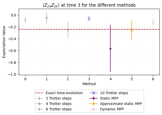
A few observations about the hardware results above:

• Going deeper is not free on hardware. The single-circuit baselines tell the story directly: the $k = 6$ circuit is essentially exact ($-0.256$ versus the reference $-0.244$), yet the deeper $k = 10$ baseline is worse ($-0.061$, off by $\sim 0.18$), not better. Once the Trotter error is already small, adding steps mostly deepens the circuit and accumulates more gate noise and decoherence. This is precisely the regime MPFs are built for: reach the accuracy of a deep circuit using only shallow constituents.

• A small-norm MPF beats the deep single circuit. The approximate-static MPF (capped at $\|x\|_1 \approx 2$) lands at $-0.259$, within $\sim 0.015$ of the reference and far closer than the $k = 10$ baseline. The dynamic MPF ($-0.127$) also comfortably beats that baseline. Both combine only the shallow $k_j = [3, 4, 6]$ circuits, yet recover an answer the deep single circuit could not.

• Coefficient norm matters more than mathematical optimality. The exact-static MPF has $\|x\|_1 = 4.66$ and is the worst estimator of all ($-0.567$, off by more than $0.3$): the large coefficient norm amplifies the residual gate noise, decoherence, and ZNE error on each $\langle A \rangle_{k_j}$ by roughly the same factor, overwhelming the Trotter-error cancellation it buys. Capping the norm (the approximate-static solver, $\|x\|_1 \approx 2$) removes this overwhelm and gives the best estimate — even though its coefficients no longer cancel the leading Trotter error exactly.

• Individual shallow circuits can still be competitive. The lone $k = 6$ constituent ($-0.256$) is itself essentially exact here — on this run it is even marginally closer than the approximate-static MPF. The catch is that you do not know in advance which single $k$ sits in the sweet spot of "converged but not yet noise-limited," and the safe-looking choice of simply going deeper ($k = 10$) to guarantee Trotter convergence is exactly the one that fails. The MPF gives a principled combination of shallow circuits that does not require guessing the right depth.

The practical takeaway is that on hardware, MPFs should be paired with strong error mitigation on each individual $\langle A \rangle_{k_j}$, the coefficient $L_1$-norm should be kept modest (use the approximate solver, or the dynamic MPF), and the Trotter steps $k_j$ should be chosen so that $t/k_{\min} \lesssim 1$ — here $k_{\min} = 3$ at $t = 3$ gives $t/k_{\min} = 1$, keeping the constituents inside the convergent regime where the leading-error model the static MPF relies on is valid. With those choices, the small-norm MPFs here match a converged single circuit while the naive "just go deeper" baseline does not, recovering the depth-versus-accuracy advantage shown in Ref. [3]. Note also that individual runs are noisy — on a different submission of the same job (or a different backend), the exact ordering can shift; the robust trends are that small-$\|x\|_1$ MPFs do well, the large-$\|x\|_1$ exact-static MPF is amplified by hardware noise, and the over-deep single circuit is noise-limited.

Next steps

References

[1] Vazquez, A. C., Egger, D. J., Ochsner, D., & Woerner, S. Well-conditioned multi-product formulas for hardware-friendly Hamiltonian simulation. Quantum, 7, 1067 (2023)

[2] Zhuk, S., Robertson, N. F., & Bravyi, S. Trotter error bounds and dynamic multi-product formulas for Hamiltonian simulation. Physical Review Research, 6(3), 033309 (2024)

[3] Robertson, N. F., et al. Tensor network enhanced dynamic multiproduct formulas. arXiv:2407.17405 (2024)