Visualization Tools (qiskit_addon_slc.visualization)

Visualization methods for shaded lightcones.

This module provides visualization methods for shaded lightcones.

animate_shaded_lightcone(circuit, bounds, coupling_map, *, reverse=False)

Animates a shaded lightcone.

This animation permits visualization of a shaded lightcone on top of a QPU’s coupling map, making interpretation of shaded lightcones easier for circuits that act on qubits with connectivity higher than a 1D line.

The qubits are placed by embedding the coupling_map into a square lattice, so that every coupling is drawn as a unit step. This works for heavy-hex and square connectivity alike and does not depend on the qubit numbering.

Parameters:

• circuit (QuantumCircuit) – the circuit whose shaded lightcone to animate.

• bounds (dict[str, PauliLindbladMap]) – the bounds to use for the shaded lightcone.

• coupling_map (CouplingMap) – the qubit connectivity map onto which to project the 1- and 2-weight bounds.

• reverse (bool) – whether to animate the circuit layers in reverse order.

Returns:

The plotly figure.

Raises:

• ValueError – if the coupling_map cannot be laid out on a grid.

• ValueError – if the bounds contain a term acting on more than 2 qubits, which has no place in the drawing.

• ValueError – if the circuit does not act on exactly the qubits of the coupling_map.

• ValueError – if none of the circuit’s boxes have bounds.

• ValueError – if the bounds contain a 2-qubit term on an uncoupled pair of qubits.

Return type:

Figure

draw_shaded_lightcone(circuit, bounds, noise_model_paulis, *, pauli_filter=None, include_empty_boxes=True, **rendering_kwargs)

Draws a shaded lightcone.

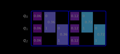
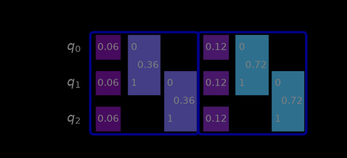
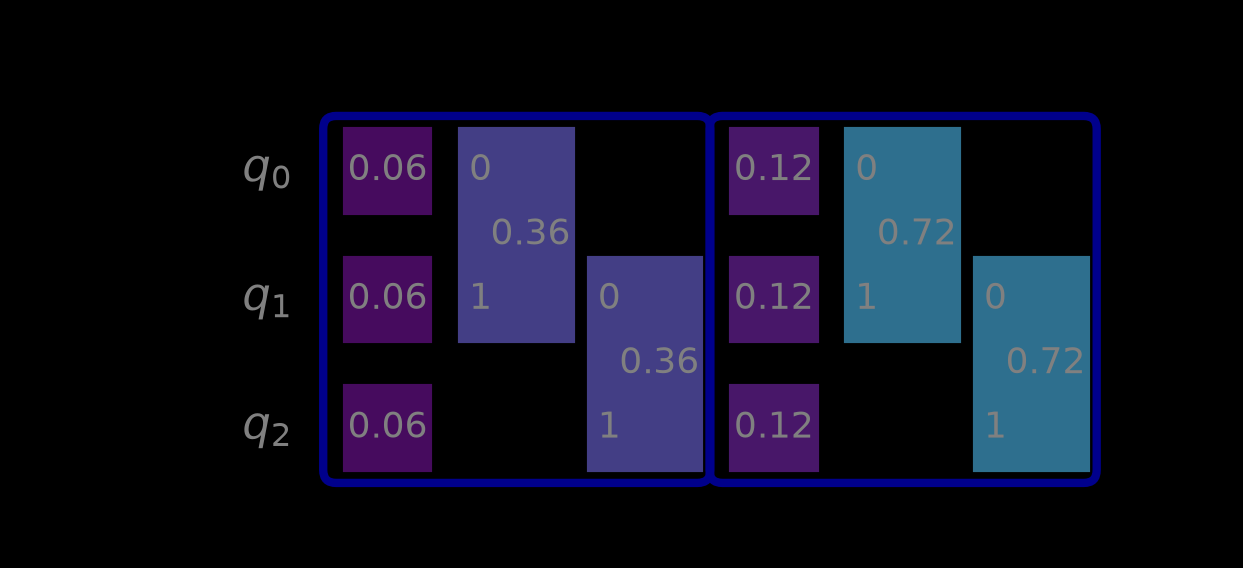
First, the provided bounds are accumulated and filtered according to pauli_filter. See also accumulate_filtered_bounds(). Then, the resulting bounds are overlaid onto the provided circuit (see overlay_bounds_onto_circuit()) and subsequently rendered (see render_bounds()).

This is the single-call entry point for the three-step pipeline; use it unless you need the intermediate results.

The noise models below come from generate_noise_model_paulis(), which produces the 1- and 2-weight Pauli terms that are actually learned for each box. The bound values are made up, with \(Z\) errors taken three times as likely as \(X\) ones so that the effect of filtering is visible.

>>> import numpy as np
>>> from qiskit import QuantumCircuit
>>> from qiskit.circuit import BoxOp
>>> from qiskit.quantum_info import PauliLindbladMap
>>> from samplomatic import InjectNoise
>>> from samplomatic.utils import find_unique_box_instructions
>>> from qiskit_addon_slc.utils import generate_noise_model_paulis
>>> from qiskit_addon_slc.visualization import draw_shaded_lightcone

>>> circuit = QuantumCircuit(3)
>>> for idx, (qubit_0, qubit_1) in enumerate([(0, 1), (1, 2)]):
...     body = QuantumCircuit(3)
...     _ = body.cx(qubit_0, qubit_1)
...     annotation = InjectNoise(ref=f"noise_{idx}", modifier_ref=f"box_{idx}")
...     _ = circuit.append(BoxOp(body, annotations=[annotation]), [0, 1, 2])

>>> noise_model_paulis = generate_noise_model_paulis(
...     find_unique_box_instructions(circuit)
... )
>>> rates = {"X": 0.01, "Y": 0.02, "Z": 0.03}
>>> bounds = {
...     f"box_{idx}": PauliLindbladMap.from_components(
...         np.array(
...             [
...                 sum(rates[pauli] for pauli in label)
...                 for label, _ in noise_model_paulis[f"noise_{idx}"].to_sparse_list()
...             ]
...         )
...         * (idx + 1),
...         noise_model_paulis[f"noise_{idx}"],
...     )
...     for idx in range(2)
... }

>>> figure = draw_shaded_lightcone(circuit, bounds, noise_model_paulis)

(png, hires.png, pdf)

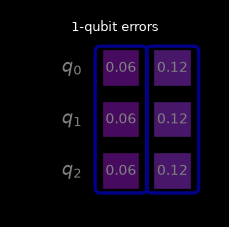
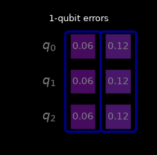
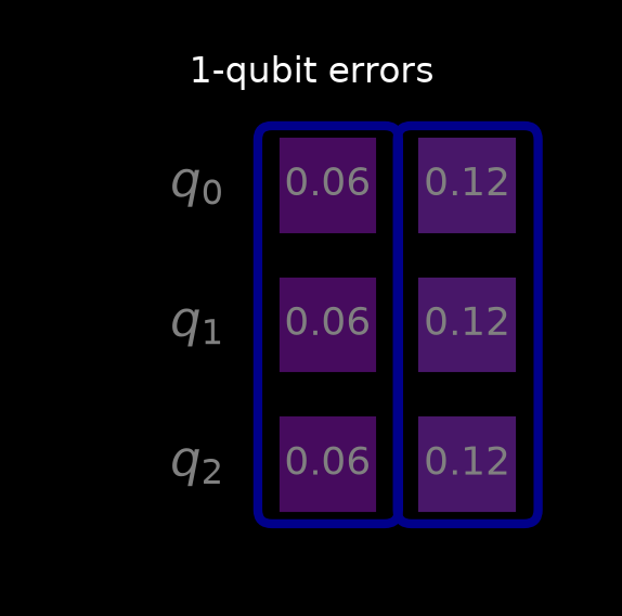
The pauli_filter is forwarded to accumulate_filtered_bounds() and also recorded in the figure title. An int selects a Pauli weight, still mixing the Pauli types:

>>> figure = draw_shaded_lightcone(
...     circuit, bounds, noise_model_paulis, pauli_filter=1
... )

(png, hires.png, pdf)

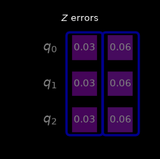
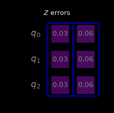
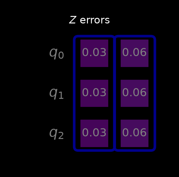
A str or Pauli matches each noise term reduced to its own non-identity support. Since the drawings above accumulate every Pauli type sharing a support, this is how to visualize one type on its own — and the two differ here by the factor of three between the \(X\) and \(Z\) rates:

>>> from qiskit_addon_slc.visualization import accumulate_filtered_bounds
>>> for pauli_filter in (None, "X", "Z"):
...     filtered = accumulate_filtered_bounds(
...         circuit, bounds, noise_model_paulis, pauli_filter=pauli_filter
...     )
...     single_qubit = {
...         support[0]: round(float(bound), 3)
...         for support, bound in sorted(filtered["box_0"].items())
...         if len(support) == 1
...     }
...     print(f"{str(pauli_filter):>4}: {single_qubit}")
None: {0: 0.06, 1: 0.06, 2: 0.06}
   X: {0: 0.01, 1: 0.01, 2: 0.01}
   Z: {0: 0.03, 1: 0.03, 2: 0.03}

>>> figure = draw_shaded_lightcone(
...     circuit, bounds, noise_model_paulis, pauli_filter="Z"
... )

(png, hires.png, pdf)

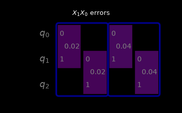
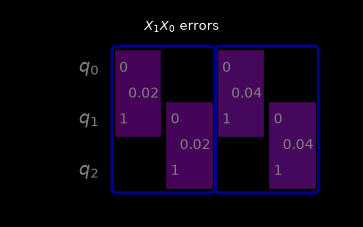
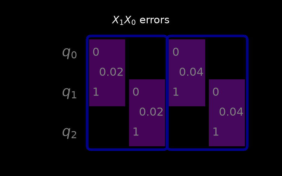
Because the match uses the reduced support, a weight-2 term is selected by "XX" rather than by a full-width label such as "XXI":

>>> figure = draw_shaded_lightcone(
...     circuit, bounds, noise_model_paulis, pauli_filter="XX"
... )

(png, hires.png, pdf)

See also

accumulate_filtered_bounds(), overlay_bounds_onto_circuit(), render_bounds()

Parameters:

• circuit (QuantumCircuit) – the circuit whose shaded lightcone to draw.

• bounds (dict[str, PauliLindbladMap]) – the bounds to use for the shaded lightcone.

• noise_model_paulis (dict[str, QubitSparsePauliList]) – the Pauli error terms of the circuit’s noise models.

• pauli_filter (Pauli | str | int | None) – the optional Pauli type by which the bounds were filtered.

• include_empty_boxes (bool) – whether to include empty boxes or not.

• rendering_kwargs – any additional keyword arguments are forwarded to QuantumCircuit.draw().

Returns:

The mpl figure.

Return type:

Figure

accumulate_filtered_bounds(circuit, bounds, noise_model_paulis, pauli_filter=None)

Accumulates the bound values filtered by a specified Pauli type.

Bound values are summed per non-identity support, so without a filter the bounds of all noise terms sharing a support are accumulated into a single value.

A str or Pauli filter is matched against each noise term reduced to its own non-identity support, not against its full-width label. Thus "X" selects every single-qubit \(X\) term regardless of which qubit it acts on, "XX" selects the weight-2 \(XX\) terms, and a full-width label such as "IXI" matches nothing.

See also

draw_shaded_lightcone() for a runnable example of the full pipeline, as well as overlay_bounds_onto_circuit() and render_bounds().

Parameters:

• circuit (QuantumCircuit) – the circuit whose bounds to accumulate.

• bounds (dict[str, PauliLindbladMap]) – the bounds whose values to accumulate.

• noise_model_paulis (dict[str, QubitSparsePauliList]) – the Pauli noise terms for each noise model.

• pauli_filter (Pauli | str | int | None) – the optional Pauli type to filter by. It behaves as follows: - None: accumulates all noise term bounds of equal support. - int: only accumulates noise term bounds of the specified Pauli weight. - str: selects noise terms whose non-identity support equals this Pauli. - Pauli: selects noise terms whose non-identity support equals this Pauli.

Returns:

A nested dictionary. The outer most key is the InjectNoise.modifier_ref (same as the original bounds). The next key is the support of the accumulated and filtered bound value (i.e. a tuple of integers). This maps to the actual bound value as a float.

Return type:

dict[str, dict[tuple[int, …], float]]

overlay_bounds_onto_circuit(pauli_bounds, circuit, *, include_empty_boxes=True)

Overlays the bounds onto the circuit.

This produces a new “QuantumCircuit” with “fake” gates reproducing those BoxOp instructions from the original circuit that had an InjectNoise annotation. Those boxes are replaced by visual representations of the computed bounds for Pauli errors of their respective support (see also accumulate_filtered_bounds()).

The returned circuit is meant for rendering only; its instructions are placeholders carrying bound values rather than executable gates.

The "max_bound" metadata entry sets the upper end of the color scale used by render_bounds(). It starts from the theoretical maximum of \(2.0\) and only grows, so it stays at \(2.0\) whenever every computed bound is tighter than that.

See also

draw_shaded_lightcone() for a runnable example of the full pipeline, as well as accumulate_filtered_bounds() and render_bounds().

Parameters:

• pauli_bounds (dict[str, dict[tuple[int, ...], float]]) – the accumulated and filtered bounds.

• circuit (QuantumCircuit) – the circuit on which to overlay the bounds.

• include_empty_boxes (bool) – whether to include empty boxes or not.

Returns:

A “fake” quantum circuit with “Gate” instructions displaying the computed bound values. The returned quantum circuit’s QuantumCircuit.metadata contains the maximum bound value under “max_bound”.

Return type:

QuantumCircuit

render_bounds(bounds_circuit, *, pauli_filter=None, **kwargs)

Renders a quantum circuit with overlaid bounds and according styling.

Each overlaid box is colored by its bound value on a viridis scale running from \(0\) to the "max_bound" metadata entry of bounds_circuit (see overlay_bounds_onto_circuit()), with a colorbar added to the right of the circuit.

Supplying the same pauli_filter that was used for accumulate_filtered_bounds() records it in the figure title, which is worth doing whenever a filtered set of bounds is rendered.

See also

draw_shaded_lightcone() for a runnable example of the full pipeline, as well as accumulate_filtered_bounds() and overlay_bounds_onto_circuit().

Parameters:

• bounds_circuit (QuantumCircuit) – the quantum circuit with overlaid bounds. See also overlay_bounds_onto_circuit().

• pauli_filter (Pauli | str | int | None) – the optional Pauli type by which the bounds were filtered. This will be indicated in the produced figure’s title.

• kwargs – any additional keyword arguments are forwarded to QuantumCircuit.draw().

Returns:

The mpl figure.

Return type:

Figure