Quimb layer-based backend (qiskit_addon_mpf.backends.quimb_layers)
A layer-wise time-evolution backend using quimb.
Warning
This backend is only available if the optional dependencies have been installed:
pip install "qiskit-addon-mpf[quimb]"
A special case of the |
|
A model for representing a layer of time-evolution interactions. |
Underlying method
This module provides a time-evolution backend similar to the TEBD-based one provided by the
quimb_tebd module. The main difference is that this module gives
the user full flexibility for defining their product formulas, thereby not limiting them to the
options built into the quimb library.
At its core, the algorithm provided by this module is still a TEBD [1] algorithm. However, rather
than enforcing the alternating updates to the even and odd bonds of the time-evolution state (see
also quimb_tebd.TEBDEvolver.sweep()) this implementation outsources the responsibility of
updating bonds in alternating fashion to the definition of multiple time-evolution layers.
This is best explained with an example. Let us assume, we have some generic Hamiltonian acting on a 1-dimensional chain of sites.
Hint
Below we are very deliberate about the order of the Hamiltonian’s Pauli terms because this directly impacts the structure of the time-evolution circuit later on.
>>> from qiskit.quantum_info import SparsePauliOp
>>> hamil = SparsePauliOp.from_sparse_list(
...     [("ZZ", (i, i+1), 1.0) for i in range(1, 9, 2)] +
...     [("Z", (i,), 0.5) for i in range(10)] +
...     [("ZZ", (i, i+1), 1.0) for i in range(0, 9, 2)],
...     num_qubits=10,
... )
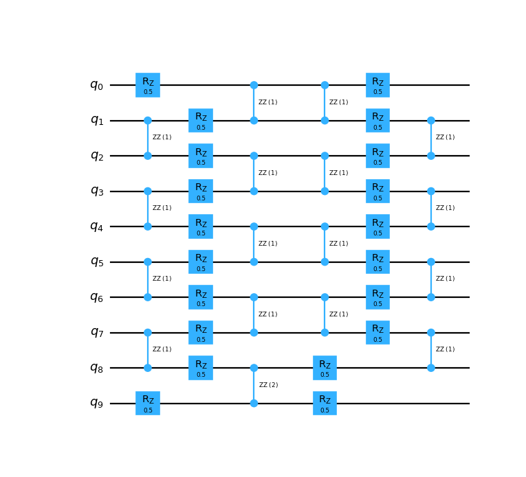
Let us now inspect the time-evolution circuit of this Hamiltonian using a second-order Suzuki-Trotter formula.
>>> from qiskit.synthesis import SuzukiTrotter
>>> from qiskit_addon_utils.problem_generators import generate_time_evolution_circuit
>>> circuit = generate_time_evolution_circuit(hamil, time=1.0, synthesis=SuzukiTrotter(order=2))
>>> circuit.draw("mpl")
<Figure size 956...x869... with 1 Axes>

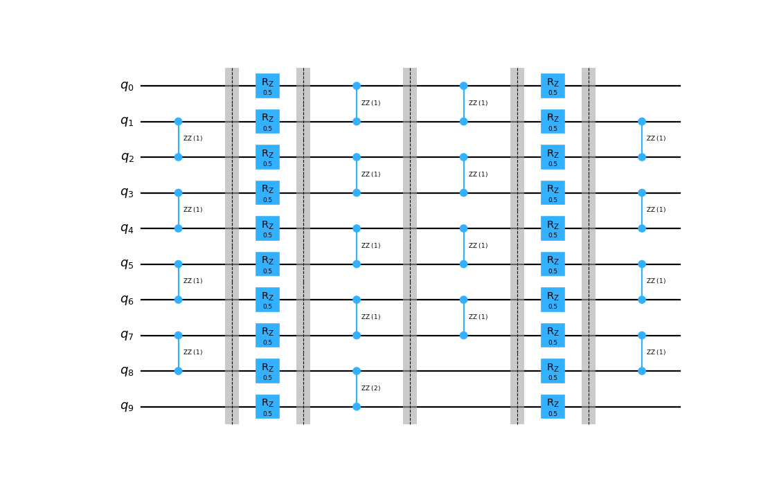
In the circuit above, we can clearly identify its layer-wise structure. We can emphasize this
further, by splitting the circuit into multiple layers as shown below (we recombine the layers
into a single circuit with barriers between them to ease the visualization).
>>> from qiskit_addon_utils.slicing import combine_slices, slice_by_gate_types
>>> layers = slice_by_gate_types(circuit)
>>> combine_slices(layers, include_barriers=True).draw("mpl")
<Figure size 1374...x869... with 1 Axes>

Hint
The asymmetry of the central layers is a result of the implementation of Qiskit’s
SuzukiTrotter formula. In its second-order form, it combines
the two half-time evolutions of the final term in the Hamiltonian into a single one of twice the
length. We could transpile this circuit to collapse all such subequent gates in the central two
layers (just like the last one), but for the sake of simplicity of this example, we will not do
that here.
It is not possible to instruct Quimb’s TEBD algorithm to simulate the exact structure of the circuit shown above. The reason for that is a limitation in its interface, as it only accepts the full Hamiltonian to be provided which is then time-evolved using pre-defined Trotter formulas. However, in doing so it does not treat the order of the Pauli terms in a Hamiltonian with any significance (like we do here).
If one wants to compute the dynamic MPF coefficients of a time-evolution employing a product formula
structure other than the ones implemented in Quimb (like the example above), then one can use the
time-evolution algorithm provided by this module. Rather than taking a single monolithic Hamiltonian
whose time-evolution is to be modeled, the LayerwiseEvolver accepts a list
of LayerModel objects, each one describing an individual layer of the
product formula. This gives the user full flexibility in defining the Trotter decomposition down to
the most granular level.
However, caution must be applied to ensure that the property of TEBD to update even and odd bonds in an alternating manner is still guaranteed. Luckily, for quantum circuits consisting of at most two-qubit gates, this property is satisfied by construction.
Code example
In this section, we build up on the example above and show how to take a custom Trotter formula and
use it to construct a LayerwiseEvolver which can be used to replace the
quimb_tebd.TEBDEvolver in the workflow described in quimb_tebd.
Hint
The overall workflow of using this module is the same as of the quimb_tebd module, so be
sure to read those instructions as well.
Simply put, we must convert each one of the circuit layers (see above) into a
LayerModel instance. For this purpose, we can use its
from_quantum_circuit() method.
>>> from qiskit_addon_mpf.backends.quimb_layers import LayerModel
>>> model0 = LayerModel.from_quantum_circuit(layers[0])
>>> layer_models = [model0]
In the code above you can see how simple the conversion is for layers which contain only two-qubit gates acting on mutually exclusive qubits (which layers of depth 1 guarantee).
However, we must be more careful with layers including single-qubit gates. The reason for that is
that the TEBD algorithm underlying the LayerwiseEvolver must update even and
odd bonds in an alternating manner. And because single-qubit gates are not applied on a site, but
instead are split in half and applied to the bonds on either side, a layer of single-qubit gates
acting on all qubits would break this assumption.
To circumvent this problem, we can take any layer consisting of only single-qubit gates, and apply twice (once on the even and once on the odd bonds).
>>> model1a = LayerModel.from_quantum_circuit(layers[1], keep_only_odd=True)
>>> model1b = LayerModel.from_quantum_circuit(layers[1], keep_only_odd=False)
>>> layer_models.extend([model1a, model1b])
Now that we know how to treat layers consisting of two-qubit and single-qubit gates, we can transform the remaining layers.
>>> for layer in layers[2:]:
...     num_qubits = len(layer.data[0].qubits)
...     if num_qubits == 2:
...         layer_models.append(LayerModel.from_quantum_circuit(layer))
...     else:
...         layer_models.append(
...             LayerModel.from_quantum_circuit(layer, keep_only_odd=True)
...         )
...         layer_models.append(
...             LayerModel.from_quantum_circuit(layer, keep_only_odd=False)
...         )
>>> assert len(layer_models) == 8
In the end, we have 8 LayerModel’s, one for each of the 4 two-qubit layers,
and two for each of the 2 single-qubit layers.
Finally, we can define our ApproxEvolverFactory protocol to be used within the
setup_dynamic_lse() function.
>>> from functools import partial
>>> from qiskit_addon_mpf.backends.quimb_layers import LayerwiseEvolver
>>> approx_evolver_factory = partial(
...     LayerwiseEvolver,
...     layers=layer_models,
...     split_opts={"max_bond": 10, "cutoff": 1e-5},
... )
Caution
It should be noted, that in this workflow we have not yet fixed the time step used by the Trotter
formula. We have also only set up a single repetition of the Trotter formula as the rest will be
done by the internal DynamicMPF algorithm, executed during setup_dynamic_lse().
Of course, you could also use this to specify a ExactEvolverFactory. But you can also
mix-and-match a quimb_layers.LayerwiseEvolver with a quimb_tebd.TEBDEvolver.
Resources
[1]: https://en.wikipedia.org/wiki/Time-evolving_block_decimation