Simulate a kicked Ising model with the TEM function

Algorithmiq's Tensor-network Error Mitigation (TEM) method is a hybrid quantum-classical algorithm designed for performing noise mitigation entirely within the classical post-processing stage. With TEM, the user can compute observables' expectation values, mitigating the inevitable noise-induced errors that occur on quantum hardware with increased accuracy and cost efficiency, making it a highly attractive option for quantum researchers and industry practitioners alike.

This tutorial demonstrates how TEM can obtain meaningful results for a quantum system's dynamics, which would be inaccessible without error mitigation and which require substantially more quantum resources if other error mitigation methods such as PEC and ZNE are used.

Usage estimate: This notebook uses approximately 10 QPU minutes on Heron r3 devices. The runtime can depend substantially on the chosen device. Per-section usage estimates can be found below.

Run error-mitigated many-body physics experiments with the TEM function

This tutorial is based on the following reference: L. E. Fischer et al., Nat. Phys. (2026). This reference discusses a real simulation on quantum hardware of up to 91 qubits. In this tutorial, we recreate a similar simulation on a smaller circuit size.

The kicked Ising model corresponds to the usual Ising model:

$\hat{H}_{\text{I}} = J \sum_{n=0}^{N-2} \hat{Z}_n \hat{Z}_{n+1} + h \sum_{n=0}^{N-1} \hat{Z}_n$

to which is applied a transverse kick:

$\hat{H}_{K} = b \sum_{n=0}^{N-1} \hat{X}_n$

The goal is to simulate the dynamics of a state under the transverse kicked Ising Hamiltonian, whose time evolution can be implemented by a Floquet unitary $\hat{U}_{\text{KI}} = e^{-i \hat{H}_K} e^{-i \hat{H}_I}$. The initial state to evolve is the one in which the first qubit is in the state $|+\rangle$, while the others are paired up and set in the Bell state $(|00\rangle + |11\rangle)/\sqrt{2}$.

The quantity we want to observe is the correlation function. The reference paper discusses how this quantity can be rewritten as an $\hat{X}$ Pauli operator on the $n^{th}$ qubit. After a number of physical time steps $t$, we compute the value of the Pauli operator $\hat{X}_{n=t}$. Depending on the system's parameters, the value of this observable is equal to a value that can be computed exactly, or only simulated through approximate methods. Specifically, for $|J|=|b|=\pi/4$ it is equal to $[\cos(2h)]^t$, which is the value we will use to benchmark the results of this tutorial. Furthermore, at a given time step $t$, $\langle\hat{X}_{n\neq t}\rangle$ is zero. For details to obtain these values, and for comparison with approximate classical simulation results outside of these parameters, see L. E. Fischer et al., Nat. Phys. (2026).

TEM works by first characterizing the noise for each unique layer of two-qubit gates in the circuit, as well as characterizing the readout error. Then, the circuit is executed on the quantum machine. Finally, the tensor network error mitigation is performed on the classical resources in IBM Cloud® and the mitigated value is returned. In this example, the circuit has two unique layers to characterize.

Setup

As a prerequisite, ensure that the necessary dependencies are installed.

%pip install numpy matplotlib qiskit qiskit-ibm-catalog qiskit-ibm-runtime pylatexenc qiskit_qasm3_import

import os
from matplotlib import pyplot as plt
import numpy as np
 
from qiskit.quantum_info import SparsePauliOp
from qiskit.qasm3 import load
 
from qiskit_ibm_catalog import QiskitFunctionsCatalog

Error mitigation with TEM

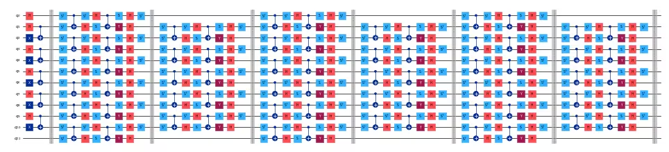
We provide here a circuit that implements the kicked Ising model described above. The circuit is prepared as follows. First, there is a state preparation phase, in which the first qubit is in the state $|+\rangle$, while the others are in Bell pairs $(|00\rangle + |11\rangle)/\sqrt{2}$. This is followed by the brickwork structure that implements the unitary evolution $\hat{U}_{\text{KI}}$. The number of physical time steps correspond to $t/2$ circuit layers.

The following code downloads the two QASM files needed for this tutorial.

# Download required QASM files
import urllib
 
urllib.request.urlretrieve(
    "https://ibm.box.com/shared/static/swy5jtq309b0xpzluzlmsmj908yphes8.qasm",
    "ki_30q.qasm",
)
urllib.request.urlretrieve(
    "https://ibm.box.com/shared/static/et3gkodonw6gsp2trs43lzaozrdtiu7s.qasm",
    "ki_12q.qasm",
)

We can visualize a small version of the circuit, with 12 qubits and six time steps:

# Parameters of the kicked Ising model
h = 0.0
num_qubits = 12
t_steps = 6
 
# Load the circuit for the kicked Ising model
small_circuit = load("ki_12q.qasm")
 
# Draw the circuit
small_circuit.draw("mpl", scale=0.25, fold=-1)

Output:

Next, build the observable, $\hat{X}_{n=t}$. It is constructed as a simple Pauli string with the order matching the one used by Qiskit:

def xt_observable(n_qubits, t_steps):
    pauli_str = "".join(["I" * t_steps, "X", "I" * (n_qubits - t_steps - 1)])
    pauli_str = pauli_str[::-1]  # Reverse the string to match qiskit order
    return SparsePauliOp(data=pauli_str, coeffs=1.0)

In our small 12-qubit example, the observable looks like this:

# Build the observable for the kicked Ising model
small_observable = xt_observable(n_qubits=12, t_steps=6)
print(small_observable)

Output:

SparsePauliOp(['IIIIIXIIIIII'],
              coeffs=[1.+0.j])

Qiskit Functions use PUBs as the way to collect the inputs. In our case, let's consider a single circuit and observable as our PUB:

# Collect the input PUBs, in this case composed of a single circuit and observable
pubs = [(small_circuit, [small_observable])]

Next, we get access to the TEM function. We first set up the required authentication to IBM Cloud and select a backend from the available devices. The token, available backends, and corresponding cloud resource names (CRN) can be obtained by logging in to your account on the IBM Quantum Platform dashboard.

# Set IBM Quantum credentials and backend configuration
personal_token = os.environ.get(
    "QISKIT_IBM_TOKEN", "<API-KEY>"
)  # Replace with your personal token or set the environment variable
channel = "ibm_quantum_platform"
crn = "your_crn"  # Replace with the Cloud Resource Name (CRN)
 
# Select the QPU backend
backend_name = "ibm_qpu_name"  # Replace with your desired backend's name

Load the TEM function from the Qiskit Functions Catalog:

# Load the TEM function from the Qiskit Functions Catalog
catalog = QiskitFunctionsCatalog(
    channel=channel,
    token=personal_token,
    instance=crn,
)
tem = catalog.load("algorithmiq/tem")

We can now run an experiment on the kicked Ising circuit with error mitigation provided by TEM. Using default settings, TEM can be run in a simple way with an expected QPU runtime of around 2.5 minutes, depending on the QPU:

tem_job = tem.run(pubs=pubs, backend_name=backend_name)

With default options, the TEM function runs three jobs on the quantum computer: noise learning, readout mitigation, and circuit sampling. The number of shots used by each of these can be changed in the options passed to the function. By default, these parameters are set to achieve a precision of 0.05 in the mitigated expectation values.

You can check the status of your job on the IBM Quantum Platform dashboard or with:

print(tem_job.status())

Output:

QUEUED

When the status is DONE, we can check the raw and mitigated results. The tem_evs defined below are the expectation values of the requested observables, in this case just one observable, $\langle \hat X_{n=t}\rangle$, and tem_std are the corresponding standard deviations.

# Get the results of the TEM job
tem_results = tem_job.result()[
    0
]  # Get the first and only result from the job
tem_evs = tem_results.data.evs[0]
tem_std = tem_results.data.stds[0]
 
print(f"TEM Result: {tem_evs:.3f} ± {tem_std:.3f}")

Output:

TEM Result: 1.031 ± 0.046

We can also check how much quantum runtime was used for each call at IBM Quantum Platform, or by inspecting the result metadata from the Python code.

# Get the TEM job runtime
tem_runtime = tem_job.result().metadata["resource_usage"][
    "RUNNING: EXECUTING_QPU"
]["QPU_TIME"]
 
print(f"TEM Runtime: {tem_runtime} seconds")

Output:

TEM Runtime: 155.0 seconds

Customize TEM parameters and advanced options

The TEM function provides several advanced options to customize your error mitigation workflow. These options allow you to control the precision, number of shots, noise learning strategies, and other parameters to better suit your experiment's requirements and available quantum resources.

Common advanced options are:

• precision: Specify the target precision for the mitigated expectation values.
• default_shots: Instead of precision, you can specify the number of shots used by the measurement job.
• tem_max_bond_dimension: The maximum bond dimension used in the tensor network.
• tem_compression_cutoff: The cutoff value to be used for the tensor network.
• noise learning options: Configure how noise is characterized, such as the number of repetitions or specific calibration circuits.
• private: Ensure that circuits and experiment results are private to you and disable multiple downloads of job results.

Refer to the TEM documentation or the Qiskit Functions Catalog for a full list of supported options and their descriptions. You can adjust these parameters to balance between runtime, resource usage, and result accuracy.

You can pass these options as a dictionary to the options argument when running the TEM function:

options = {
    "default_shots": 10_000,
    "tem_max_bond_dimension": 512,
    "tem_compression_cutoff": 1e-16,
    "compute_shadows_bias_from_observable": True,  # This option helps optimizing the measurement
    # stage since the observable is strongly biased toward the X operator for all the qubits.
    "private": False,  # set to True to keep experiment results private, recommended for confidential circuits
}

Custom options for the noise learner can also be passed. They follow the definitions used in the Qiskit Runtime NoiseLearnerOptions:

nl_options = {
    "num_randomizations": 32,
    "max_layers_to_learn": 2,
    "shots_per_randomization": 128,
    "layer_pair_depths": [0, 1, 2, 4, 16, 32],
}
 
# add noise learning options to the overall options
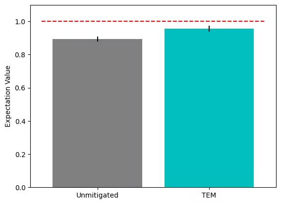
options |= nl_options

Re-run the experiment with these custom options tuned to our circuit. The expected runtime is approximately four QPU minutes.

tem_job_custom = tem.run(
    pubs=pubs, backend_name=backend_name, options=options
)

If the job is not set as private, we can recover the result at a later point. To do so, save the job ID printed here and use tem_job_custom = catalog.get_job_by_id("your-job-id").

job_id = tem_job_custom.job_id
print(f"Job ID: {job_id}")

Output:

Job ID: 1ba10094-a541-457a-9287-dbd49306d12d

results_custom = tem_job_custom.result()
tem_evs = results_custom[0].data.evs[0]
tem_std = results_custom[0].data.stds[0]
 
print(f"TEM Result: {tem_evs:.3f} ± {tem_std:.3f}")

Output:

TEM Result: 0.956 ± 0.018

We can now inspect the results and the metadata to get insight into the experiment:

metadata_custom = results_custom[0].metadata
 
unmitigated_evs = metadata_custom["evs_non_mitigated"][0]
unmitigated_stds = metadata_custom["stds_non_mitigated"][0]
print(f"Unmitigated Result: {unmitigated_evs:.3f} ± {unmitigated_stds:.3f}")
 
# Exact result for the kicked Ising model from the reference paper
exact_evs = np.cos(2 * h) ** t_steps
print("Exact Result:", exact_evs)

Output:

Unmitigated Result: 0.894 ± 0.015
Exact Result: 1.0

# Plot comparing the different expectation values
plt.bar(
    ["Unmitigated", "TEM"],
    [unmitigated_evs, tem_evs],
    yerr=[unmitigated_stds, tem_std],
    color=["grey", "c"],
)
plt.hlines(y=exact_evs, xmin=-0.5, xmax=1.5, colors="r", linestyles="dashed")
plt.ylabel("Expectation Value")
plt.ylim(0, 1.1)
plt.show()

Output:

Finally, we can check the impact of the custom options on QPU and classical runtime:

# Get the metadata of the TEM job
job_metadata = results_custom.metadata
 
# Get the runtime of the TEM job
qpu_runtime = job_metadata["resource_usage"]["RUNNING: EXECUTING_QPU"][
    "QPU_TIME"
]
classical_runtime = (
    job_metadata["resource_usage"]["RUNNING: OPTIMIZING_FOR_HARDWARE"][
        "CPU_TIME"
    ]
    + job_metadata["resource_usage"]["RUNNING: POST_PROCESSING"]["CPU_TIME"]
)
 
print(f"QPU Runtime: {qpu_runtime} seconds")
print(f"Classical Runtime: {classical_runtime} seconds")

Output:

QPU Runtime: 342.0 seconds
Classical Runtime: 107.632604 seconds

Scale TEM to large circuits

Large circuits can, in principle, be run with the TEM function. However, it is important to be aware of the of the limitations of the classical resources, as TEM is executed on IBM Cloud runners with potentially very long run times. For extremely large circuits, contact the TEM support team at qiskit_ibm@algorithmiq.fi.

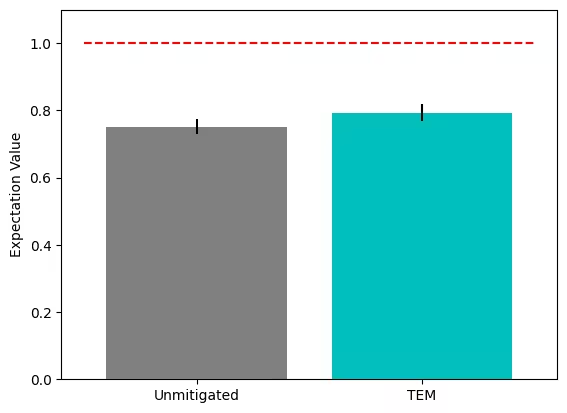
Here we run an example with a larger, utility-scale-sized 30-qubit circuit, optimizing the TEM parameters for speed rather than accuracy.

# Kicked Ising model parameters
n_qubits = 30
t_steps = 15
h = 0.0
 
# Load the circuit for the kicked Ising model
circuit = load("ki_30q.qasm")
 
 
# Build the observable for the kicked Ising model
observable = xt_observable(n_qubits=n_qubits, t_steps=t_steps)
 
# Collect the input PUBs, in this case composed of a single circuit and observable
pubs = [(circuit, [observable])]

Let's define some performance-oriented options:

options = {
    "num_randomizations": 32,
    "max_layers_to_learn": 2,
    "shots_per_randomization": 128,
    "layer_pair_depths": [0, 1, 2, 4, 16, 32, 64],
    "default_shots": 5_000,
    "tem_max_bond_dimension": 128,
    "tem_compression_cutoff": 1e-10,
    "compute_shadows_bias_from_observable": True,
    "private": False,
}

Finally, run the experiment, get the result, and visualize it. This will take approximately 3.5 QPU minutes.

tem_job_large = tem.run(pubs=pubs, backend_name=backend_name, options=options)

job_id = tem_job_large.job_id
print(f"Job ID: {job_id}")

Output:

Job ID: 9f3f190f-f4b0-4dcb-bb83-5f71f37d0d77

results_large = tem_job_large.result()
tem_evs = results_large[0].data.evs[0]
tem_std = results_large[0].data.stds[0]
 
print(f"TEM Result: {tem_evs:.3f} ± {tem_std:.3f}")
 
 
# Get the metadata of the TEM job
job_metadata = tem_job_large.result().metadata
 
# Get the runtime of the TEM job
qpu_runtime = job_metadata["resource_usage"]["RUNNING: EXECUTING_QPU"][
    "QPU_TIME"
]
classical_runtime = (
    job_metadata["resource_usage"]["RUNNING: OPTIMIZING_FOR_HARDWARE"][
        "CPU_TIME"
    ]
    + job_metadata["resource_usage"]["RUNNING: POST_PROCESSING"]["CPU_TIME"]
)
 
print(f"QPU Runtime: {qpu_runtime} seconds")
print(f"Classical Runtime: {classical_runtime} seconds")

Output:

TEM Result: 0.794 ± 0.026
QPU Runtime: 203.0 seconds
Classical Runtime: 251.71805499999996 seconds

# Plot comparing the different expectation values
metadata_large = results_large[0].metadata
unmitigated_evs = metadata_large["evs_non_mitigated"][0]
unmitigated_stds = metadata_large["stds_non_mitigated"][0]
 
exact_evs = np.cos(2 * h) ** t_steps
 
plt.bar(
    ["Unmitigated", "TEM"],
    [unmitigated_evs, tem_evs],
    yerr=[unmitigated_stds, tem_std],
    color=["grey", "c"],
)
plt.hlines(y=exact_evs, xmin=-0.5, xmax=1.5, colors="r", linestyles="dashed")
plt.ylabel("Expectation Value")
plt.ylim(0, 1.1)
plt.show()

Output: