Work with fermionic circuits
Important
The concepts in this guide are currently available only in the Python API. Equivalent functionality will be made available in the C API in a future release.
This guide explains how to use the FermionicCircuit to implement
quantum algorithms directly in fermionic space, rather than mapping to qubits
first.
Why use fermionic circuits
Consider the traditional workflow for implementing the time evolution of a fermionic Hamiltonian on a qubit-based architecture:
Define the fermionic Hamiltonian (for example, \(H = \sum_{pq} h_{pq} c^\dagger_p c_q\)).
Map it to a qubit operator (for example, by using the Jordan-Wigner mapping).
Implement the time evolution in qubit space (using Trotterization or other methods).
This approach has a fundamental limitation; early mapping to qubits discards problem-aware knowledge about the fermionic structure. Standard optimization passes cannot exploit fermionic symmetries or allowed term reorderings, resulting in suboptimal circuits with unnecessary depths and gate counts.
The FermionicCircuit enables a better workflow:
Define the fermionic Hamiltonian (for example, \(H = \sum_{pq} h_{pq} c^\dagger_p c_q\)).
Implement the time evolution directly in fermionic space using fermionic gates.
Map to qubit space as part of the transpilation process.
This approach addresses the limitation by keeping problem-aware knowledge in fermionic space, where optimization passes can exploit fermionic structure and commutation relations to reduce circuit depth. The fermionic circuit describes what computation to perform, while transpilation handles how to map it to qubits, providing a cleaner separation of concerns.
Generic mode indexing
Both the operators module and the
FermionicCircuit use generic mode-based indexing that makes no
assumptions about the nature of the modes. A mode is simply an abstract index
labeling a fermionic degree of freedom, with no inherent semantics. This design
choice mirrors the operators module and ensures maximum flexibility.
For example, you can implement time evolution for any operator implementing the
OperatorTrait protocol, regardless of its mathematical representation.
Build a fermionic circuit
The example below implements the time evolution described in the previous section.
It constructs a FermionicCircuit by specifying the number of fermionic
modes, then adds fermionic gates from the qiskit_fermions.circuit.library
to implement the time evolution.
The example also demonstrates how to incorporate domain knowledge into an operator by using operator term grouping. By assigning group indices to the Hamiltonian terms, you preserve structural information that optimization passes can exploit throughout the transpilation stack.
>>> from qiskit_fermions.circuit import FermionicCircuit
>>> from qiskit_fermions.circuit.library import Evolution
>>> from qiskit_fermions.operators import FermionOperator, cre, ann
>>>
>>> # Create a circuit with 4 fermionic modes
>>> circuit = FermionicCircuit(4)
>>>
>>> # Define a simple fermionic Hamiltonian
>>> hamiltonian = FermionOperator.from_terms([
...     ([cre(0), ann(2)], 0.5),
...     ([cre(2), ann(0)], 0.5),
...     ([cre(1), ann(3)], 0.5),
...     ([cre(3), ann(1)], 0.5),
... ])
>>> # Add some problem structure by grouping our Hamiltonian terms
>>> hamiltonian.groups = [0, 0, 1, 1]
>>>
>>> # Add an evolution gate to implement exp(-i * t * H)
>>> evolution = Evolution(4, hamiltonian, time=1.0)
>>> circuit.append(evolution, circuit.register)
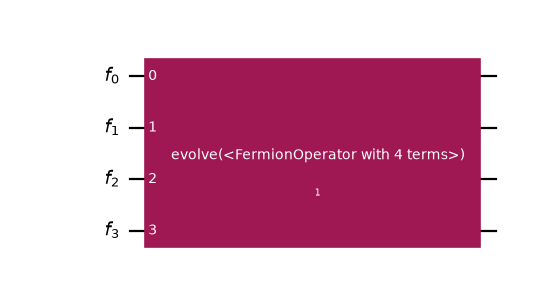
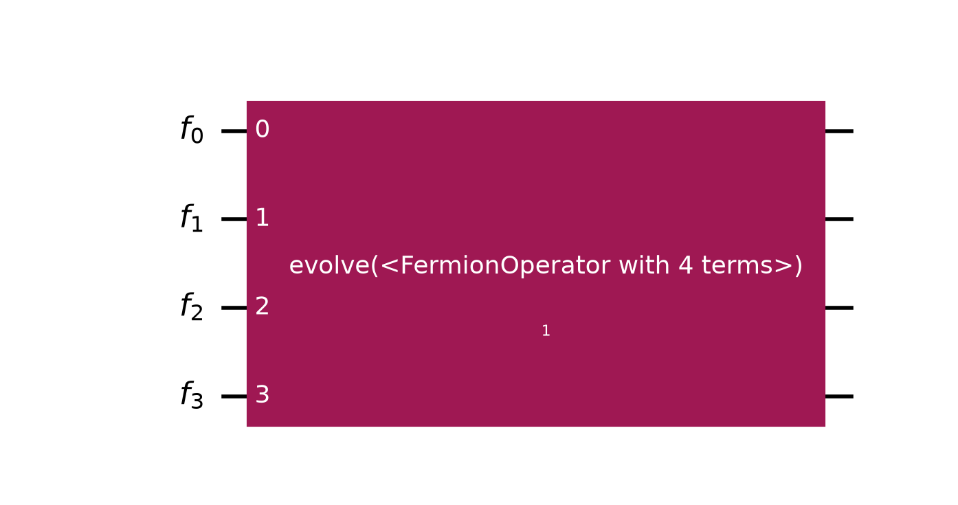
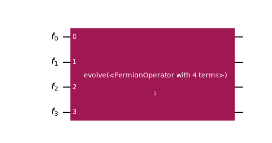
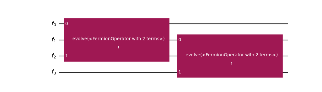
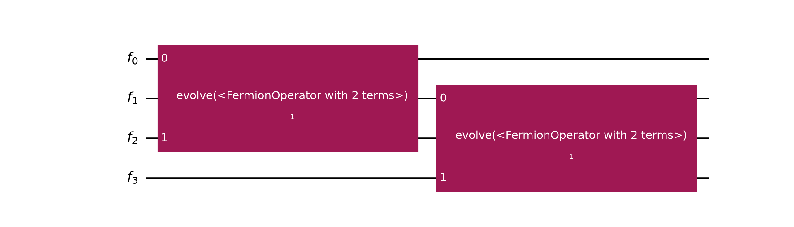
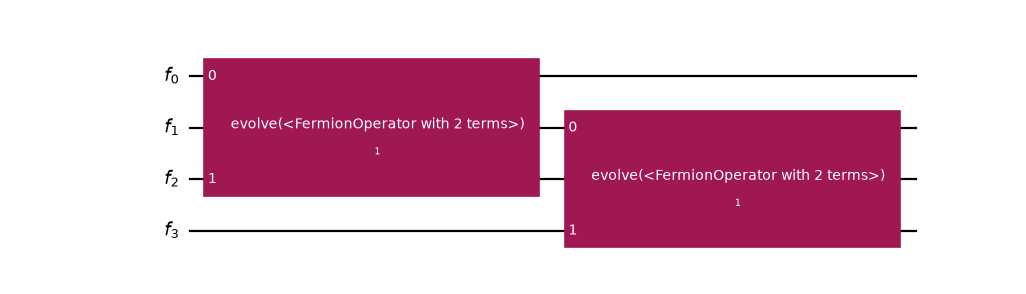
Notice how the operator term grouping is preserved even in simple operations like decomposition. This demonstrates how structural information flows through the circuit stack. To understand the full transpilation to qubits, refer to the Transpiling fermionic circuits guide.
Keep gates apart with a barrier
The optimization passes fuse neighboring gates where they can. For example,
MergeOrbitalRotations combines a run of consecutive
OrbitalRotation gates into one, and
MergeSlaterDeterminantPreparation folds an InitializeModes
into the rotation that follows it.
Use FermionicCircuit.barrier() when you want to prevent that. A barrier
carries no unitary effect, so it does not change the state your circuit
prepares; it only marks a point that the passes do not fuse across. Call it
without arguments to span every mode, or pass the modes to restrict it to:
>>> from qiskit_fermions.circuit.library import OrbitalRotation
>>> import numpy as np
>>>
>>> rotations = FermionicCircuit(4)
>>> rotations.append(OrbitalRotation(np.eye(4, dtype=complex)), rotations.register)
>>> rotations.barrier()
>>> rotations.append(OrbitalRotation(np.eye(4, dtype=complex)), rotations.register)
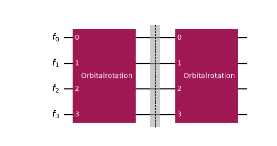
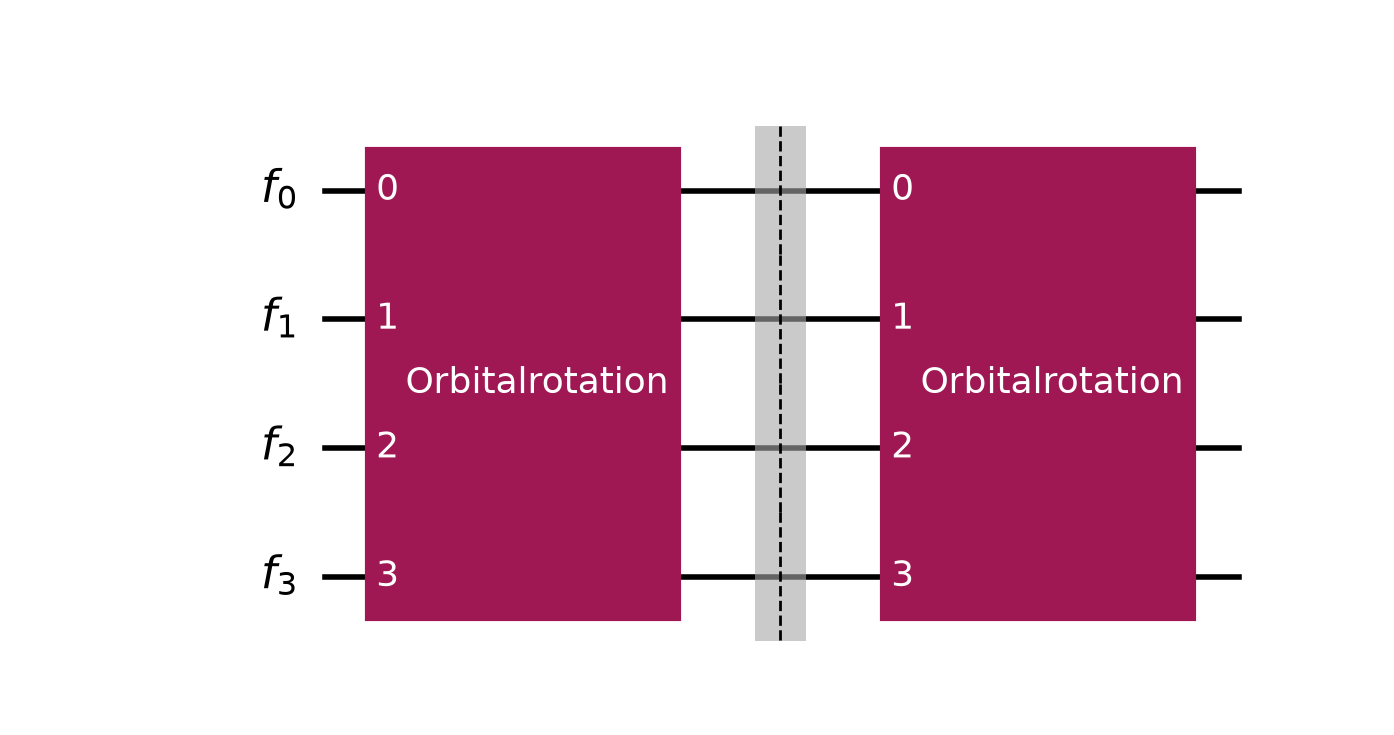
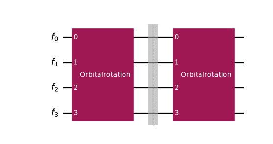
Barriers survive the fermion-to-qubit transpilation, so they also constrain the qubit-level optimization that follows. The Transpile fermionic circuits guide covers that stage.
Repeat a circuit
Many algorithms apply the same block of gates many times over. Time evolution is
the common case: a Trotter step is built once, then repeated to reach the target
time. Use repeat() to build the repeated circuit, and
compose() to join it to a state preparation prefix.
The example below builds a second-order Trotter step for a Fermi-Hubbard model.
The step is symmetric: it splits the hopping term into two half-duration
OrbitalRotation gates surrounding the on-site interaction.
>>> import scipy.linalg
>>> from qiskit_fermions.circuit.library import InitializeModes, OrbitalRotation
>>>
>>> norb, reps, time = 2, 3, 1.0
>>> num_modes = 2 * norb
>>> dt = time / reps
>>>
>>> hopping = np.zeros((norb, norb))
>>> hopping[0, 1] = hopping[1, 0] = -1.0
>>> interaction = FermionOperator.from_dict(
...     {(cre(p), ann(p), cre(p + norb), ann(p + norb)): 2.0 for p in range(norb)}
... )
>>>
>>> def rotation(duration):
...     propagator = scipy.linalg.expm(-1j * duration * hopping)
...     # the same rotation acts on the alpha and beta halves of the register
...     return scipy.linalg.block_diag(propagator, propagator)
>>>
>>> trotter_step = FermionicCircuit(num_modes)
>>> trotter_step.append(OrbitalRotation(rotation(dt / 2)), trotter_step.modes)
>>> trotter_step.append(
...     Evolution(num_modes, interaction, dt, atomic=True), trotter_step.modes
... )
>>> trotter_step.append(OrbitalRotation(rotation(dt / 2)), trotter_step.modes)
Repeating the step and composing it onto a Hartree-Fock reference gives the full evolution:
>>> evolution = FermionicCircuit(num_modes)
>>> evolution.append(InitializeModes([True, False, True, False]), evolution.modes)
>>> evolution.compose(trotter_step.repeat(reps), inplace=True)
>>> evolution.count_ops()["OrbitalRotation"]
6



The repetitions are flattened into the returned circuit rather than wrapped in a
single gate, so count_ops() counts two rotations per
step. That flattening is what makes the redundancy at the step boundaries
visible to the transpiler: the trailing half-duration rotation of one step and
the leading one of the next are adjacent, so
MergeOrbitalRotations combines them into a single rotation.
>>> from qiskit_fermions.transpiler import FermionicPassManager
>>> from qiskit_fermions.transpiler.passes import MergeOrbitalRotations
>>>
>>> merged = FermionicPassManager([MergeOrbitalRotations()]).run(evolution)
>>> merged.count_ops()["OrbitalRotation"]
4



The result costs one rotation per step plus one, which is what you get by fusing those half-steps by hand. Writing the step in its natural symmetric form and repeating it produces the same circuit, so the fusion is left to the optimization stage.
When you need the repetitions kept apart, pass insert_barriers=True to place
a barrier() between them. The optimization passes do
not fuse gates across a barrier, so every rotation survives:
>>> separated = trotter_step.repeat(reps, insert_barriers=True)
>>> FermionicPassManager([MergeOrbitalRotations()]).run(separated).count_ops()[
...     "OrbitalRotation"
... ]
6



Note
The reps argument of FermionicSuzukiTrotter is a different
concept. It subdivides a single Evolution gate into more, shorter
factors, whereas repeat() duplicates whole circuits.
Repeating a circuit that holds one Evolution only multiplies its
total evolution time.
Measure fermionic modes
measure_all() reads every mode out into a classical bit
of its own, pairing mode i with bit i. Use
measure() with your own
ClassicalRegister to read out only some of them.
>>> measured = trotter_step.measure_all(inplace=False)
>>> measured.count_ops()["measure"]
4
Passing inplace=False returns a measured copy and leaves the original alone,
which matters because a measurement is not unitary: a circuit carrying one can no
longer be applied to a state vector, so keep an unmeasured circuit around if you
also want to simulate it.
Measuring here, rather than on the transpiled
QuantumCircuit, is what keeps the sampled bitstrings easy
to read. A fermionic measurement names the mode it reads, so every stage that
moves modes around (RelabelModes at the fermionic level, layout and
routing at the qubit level) carries the measurement along with it, and the
bitstring stays indexed by the mode you asked about.
Note
Unlike measure_all(), no
barrier() is inserted before the measurements. Call
barrier() yourself first if you want one there.
Whether a measured bit means what you expect depends on the fermion-to-qubit
encoding, which is chosen during transpilation rather than here. Under an
occupation-basis encoding such as Jordan-Wigner each mode is carried by one
qubit and the bit is that mode’s occupation; see FermionicMeasure.
Transpile fermionic circuits
To implement the quantum algorithm represented by your
FermionicCircuit it must be transpiled to a
QuantumCircuit. You can learn how to do this in the
Transpile fermionic circuits guide.
Next steps
Learn about available fermionic gates in the
qiskit_fermions.circuit.librarydocumentation.Explore the operators explanation guide to understand how to construct fermionic Hamiltonians that you can use with fermionic circuits.
Review the SQDRIFT getting started guide for a practical end-to-end example.
Read the ffsim relationship guide to understand how a
FermionicCircuitcan be simulated directly, and how these generic mode indices take on spin semantics only at simulation time.