Simulate Bose-Hubbard dynamics with a choice of encoding

This guide builds a circuit for the time dynamics of the one-dimensional Bose-Hubbard model, from writing down the Hamiltonian to checking the evolved site densities against an exact reference. What makes the route interesting is a single idea:

Do not choose a boson-to-qubit encoding when you build the circuit. Build the circuit on bosonic modes, and let the transpiler decide how those modes become qubits.

For bosons, you nearly always need to defer the encoding. A bosonic mode holds arbitrarily many particles, so its Fock space is infinite-dimensional and no encoding exists until you first pick a truncation \(d\) (the number of occupation levels you keep). In code the truncation is given as the largest occupation a mode can hold, max_occupation \(= d - 1\), so a mode that keeps the levels \(0, 1, 2\) has max_occupation = 2 and \(d = 3\).

That makes the truncation a parameter of the encoding, not of the physics, and it is a parameter you want to vary: too small and the answer is wrong, too large and the circuit is needlessly wide. If you defer the encoding to transpile time, you can sweep the truncation without changing the circuit, the Hamiltonian, or the grouping.

See also

The operators guide for the operator data structure, the mappers guide for the encodings and the recipe for writing a custom mapper, and the transpilation guide for the transpiler stages referenced throughout.

Truncation, and what it costs

When you truncate a mode to \(d\) levels, you break the canonical commutator on the highest retained level [1], so no encoding is an isomorphism of algebras: a bosonic encoding maps states, and operators acting within the truncated subspace. Two consequences matter for everything that follows:

1. \(d\) must bound the occupation reachable by the dynamics, not merely that of the initial state.

2. Mapping does not commute with normal ordering, so decide once whether your Hamiltonian is defined in normal-ordered form, and stay consistent.

The mappers guide derives the defect and shows both consequences on running code.

1. The Hamiltonian

The Bose-Hubbard model on a lattice with bonds \(\langle i j \rangle\) is

\[H = -t \sum_{\langle i j \rangle} \left(b^\dagger_i b_j + b^\dagger_j b_i\right) + \frac{U}{2} \sum_i n_i (n_i - 1) \, ,\]

with \(n_i = b^\dagger_i b_i\). The interaction counts pairs of bosons on a site, so it requires a site to hold two particles at once. Normal-ordered, \(n_i(n_i-1) = b^\dagger_i b^\dagger_i b_i b_i\), which is the form used in what follows.

The geometry enters only through the edge list, so nothing is specific to a chain:

>>> from qiskit_bosons.operators import BosonOperator, ann, cre
>>>
>>> def bose_hubbard(edges, num_sites, tunneling, interaction):
...     """Build the normal-ordered Bose-Hubbard Hamiltonian on an arbitrary lattice."""
...     terms = {}
...     for i, j in edges:
...         terms[(cre(i), ann(j))] = -tunneling
...         terms[(cre(j), ann(i))] = -tunneling
...     for i in range(num_sites):
...         # U/2 * n_i (n_i - 1), already normal-ordered
...         terms[(cre(i), cre(i), ann(i), ann(i))] = 0.5 * interaction
...     return BosonOperator.from_dict(terms)
>>>
>>> num_sites = 4
>>> edges = [(i, i + 1) for i in range(num_sites - 1)]
>>> hamiltonian = bose_hubbard(edges, num_sites, tunneling=1.0, interaction=2.0)
>>> print(f"Number of terms: {len(hamiltonian)}")
Number of terms: 10

Two properties are worth checking first. The Hamiltonian must be Hermitian for \(e^{-itH}\) to be unitary, and it conserves the total boson number:

>>> hamiltonian.is_hermitian()
True
>>> hamiltonian.conserves_particle_number()
True

Now the bosonic question: how many levels does this operator demand?

>>> hamiltonian.max_occupation()
2

The interaction term applies two creation operators to one mode, so a mode has to hold two bosons for the term to act at all. That is a maximum occupation of 2, which is the number that LevelSpec takes as its max_occupation. A mode that keeps the occupations \(0, 1, 2\) has \(d = \texttt{max\_occupation} + 1 = 3\) levels, so max_occupation >= 2 is the same requirement as \(d \geq 3\).

This is a lower bound only: it comes from one application of the operator, and repeated application over a time evolution can reach further. It rules out cutoffs that are certainly too small, and step 6 settles, for this model and state, how large the cutoff has to be. mode_occupations() reports the bound for each mode separately, which is what a per-mode cutoff is compared against.

2. Group before mapping

The evolution is Trotterized, and how the Hamiltonian is partitioned decides what the synthesis is handed. Two considerations pull in the same direction.

First, a physical one: the individual hopping term \(b^\dagger_i b_j\) is not Hermitian. Only the pair \(b^\dagger_i b_j + b^\dagger_j b_i\) is. If you evolve under a single non-Hermitian term, the operation is not unitary, and the mapped operator would carry complex coefficients that PauliEvolutionGate rejects. Each bond’s two hopping terms must therefore stay together.

Second, an efficiency one: all the on-site interaction terms are diagonal in the occupation basis and mutually commute, so they can share a single group and be synthesized together. The same holds for the bonds that touch no common site. On a chain, every second bond is such a set: bonds 0 and 2 act on disjoint pairs of modes, so their hopping terms commute and can share a group, and bond 1 forms a group of its own. If you group the even and the odd bonds, you therefore need three groups, where one group per bond needs four. Fewer groups mean fewer factors, and also a shallower circuit: with the Gray code at max_occupation = 2 the two-qubit depth is 95 against 139. The lattice decides which bonds can share a group, which is why the partition is chosen here.

The groups attribute carries that decision into the circuit: an Evolution gate over a grouped operator decomposes into one sub-evolution per group. The partition is chosen at the bosonic level, while the lattice structure is still visible, and it survives untouched through the mapping. The grouping guide covers the checks a grouping should pass.

>>> def group_of(actions, edges):
...     """Assign each term to the even bonds, the odd bonds, or the on-site group."""
...     creations = sorted(mode for action, mode in actions if action)
...     annihilations = sorted(mode for action, mode in actions if not action)
...     if creations == annihilations:
...         return 2  # diagonal: the on-site interaction group
...     bond = tuple(sorted(set(creations) | set(annihilations)))
...     return edges.index(bond) % 2  # bonds 0 and 2 share a group, bond 1 has its own
>>>
>>> hamiltonian.groups = [group_of(actions, edges) for actions, _ in hamiltonian.iter_terms()]
>>> hamiltonian.num_groups()
3

Every group must itself be Hermitian, which is what the preceding pairing buys. groups_are_hermitian() checks all groups in one call:

>>> from qiskit_bosons.operators.terms import groups_are_hermitian
>>> groups_are_hermitian(hamiltonian)
[True, True, True]

To see what each group holds, separate the groups:

>>> for index, group in enumerate(hamiltonian.split_out_groups()):
...     print(f"group {index}: {len(group)} terms, hermitian={group.is_hermitian()}")
group 0: 4 terms, hermitian=True
group 1: 2 terms, hermitian=True
group 2: 4 terms, hermitian=True

The even-and-odd grouping is a choice, and the alternative is easy to measure. If you give every bond a group of its own, you need four groups, and the same circuit then costs more two-qubit depth. The depth is counted after the circuit is lowered with the Gray code at max_occupation = 2, which step 4 explains:

>>> from qiskit.transpiler import PassManager
>>> from qiskit_bosons.circuit import BosonicCircuit
>>> from qiskit_bosons.circuit.library import Evolution
>>> from qiskit_bosons.mappers import LevelSpec
>>> from qiskit_bosons.transpiler.presets import generate_preset_occupation_pass_manager
>>>
>>> def two_qubit_depth(operator):
...     """The two-qubit depth of one evolution under ``operator``, lowered with the Gray code."""
...     probe = BosonicCircuit(num_sites)
...     probe.append(Evolution(num_sites, operator, time=0.4), probe.modes)
...     pass_manager = generate_preset_occupation_pass_manager(LevelSpec(2, "gray"))
...     pass_manager.qubit = PassManager()
...     lowered = pass_manager.run(probe.decompose())
...     return lowered.decompose(reps=6).depth(lambda instruction: len(instruction.qubits) == 2)
>>>
>>> per_bond = bose_hubbard(edges, num_sites, tunneling=1.0, interaction=2.0)
>>> per_bond.groups = [
...     len(edges) if sorted(m for a, m in actions if a) == sorted(m for a, m in actions if not a)
...     else edges.index(tuple(sorted({m for _, m in actions})))
...     for actions, _ in per_bond.iter_terms()
... ]
>>> per_bond.num_groups(), two_qubit_depth(per_bond)
(4, 139)
>>> hamiltonian.num_groups(), two_qubit_depth(hamiltonian)
(3, 95)

3. The bosonic circuit

Note what is absent from the circuit. There is no truncation, no encoding, and no qubit count. It acts on four bosonic modes:

>>> from qiskit_bosons.circuit import BosonicCircuit
>>> from qiskit_bosons.circuit.library import Evolution, InitializeModes
>>>
>>> total_time = 0.4
>>> occupation = [1, 1, 0, 0]  # one boson on each of the first two sites
>>>
>>> circuit = BosonicCircuit(num_sites)
>>> circuit.append(InitializeModes(occupation), circuit.modes)
>>> circuit.append(Evolution(num_sites, hamiltonian, time=total_time), circuit.modes)
>>> dict(circuit.count_ops())
{'InitializeModes': 1, 'Evolution': 1}

(png, hires.png, pdf)

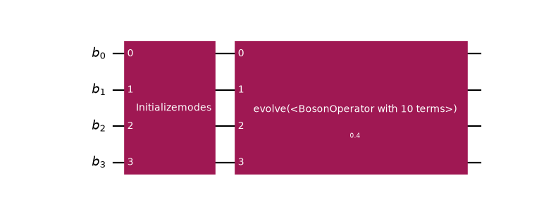
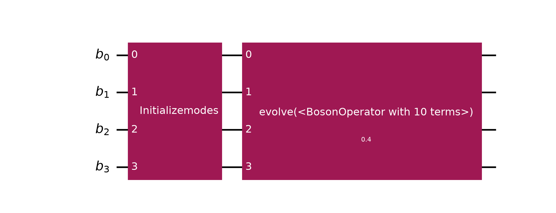
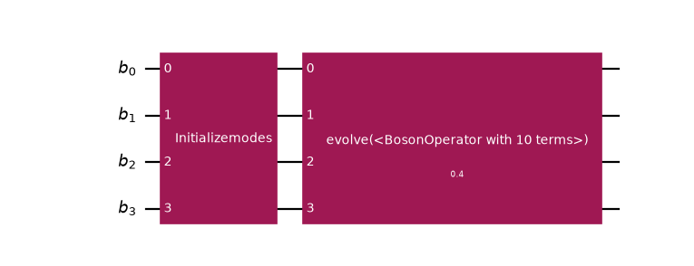
The wires are bosonic modes, not qubits. Note that InitializeModes takes integers, not flags: a mode can hold any number of bosons, so a Fock state is a list of occupation numbers.

A single decompose() turns the grouping from step 2 into one gate per group:

>>> decomposed = circuit.decompose()
>>> dict(decomposed.count_ops())
{'Evolution': 3, 'InitializeModes': 1}

(png, hires.png, pdf)

The first group holds the bonds on modes 0 and 1 and on modes 2 and 3, so its gate spans all four modes, and so does the on-site group. The middle bond has a gate of its own on modes 1 and 2.

Skip that decomposition and the grouping is simply ignored. Which method does the splitting is the synthesis of the gate, with BosonicLieTrotter as the default; Synthesize an Evolution gate in bosonic space shows the alternatives.

4. Choose the encoding at transpile time

Here is the payoff. The same circuit is lowered four times, under four different LevelEncoding values, by changing one argument. A LevelSpec pairs the encoding with the truncation of every mode, and the following preset derives the layout, the state preparation, and the operator mapping from that one spec (see Describe the truncation with a LevelSpec). A string such as "gray" is accepted wherever a LevelEncoding is.

>>> from qiskit.transpiler import PassManager
>>> from qiskit_bosons.mappers import LevelEncoding, LevelSpec
>>> from qiskit_bosons.transpiler.presets import generate_preset_occupation_pass_manager
>>>
>>> max_occupation = 2  # the largest occupation per mode, so d = max_occupation + 1 = 3 levels
>>>
>>> encodings = (
...     LevelEncoding.UNARY_PROJECTED,
...     LevelEncoding.UNARY_UNPROJECTED,
...     LevelEncoding.STANDARD_BINARY,
...     LevelEncoding.GRAY,
... )
>>> for encoding in encodings:
...     pass_manager = generate_preset_occupation_pass_manager(
...         LevelSpec(max_occupation, encoding)
...     )
...     pass_manager.qubit = PassManager()  # keep the circuit as the pipeline synthesized it
...     qubit_circuit = pass_manager.run(decomposed)
...     basis = qubit_circuit.decompose(reps=6)
...     two_qubit = basis.depth(lambda instruction: len(instruction.qubits) == 2)
...     print(f"{encoding!s:18s} qubits={qubit_circuit.num_qubits:2d}  2q-depth={two_qubit:4d}")
unary_projected    qubits=12  2q-depth= 645
unary_unprojected  qubits=12  2q-depth= 383
standard_binary    qubits= 8  2q-depth= 218
gray               qubits= 8  2q-depth=  95

These numbers contradict a natural guess. The unary encodings use \(d\) qubits per mode against \(\lceil \log_2 d \rceil\) for the compact codes, and at \(d = 3\) the compact codes win on both axes at once: fewer qubits and far fewer entangling gates. The two unary variants differ in the operator they emit, not in their layout: LevelEncoding.UNARY_PROJECTED carries a projector on every other qubit of a mode, which makes it the most expensive of the four to evolve, and LevelEncoding.UNARY_UNPROJECTED leaves the projectors out and agrees with it on the one-hot subspace. The mappers guide shows the two operators side by side, and explains why the Gray code beats standard binary (SB) on the hopping terms.

Sawaya et al. report the same ordering [2]:

though the unary code tends to require more qubits but fewer operations, it is often the case that the SB or Gray code is more efficient both in terms of qubit counts and operation counts

Their conclusion is that the best code depends on the Hamiltonian and on \(d\), which is the strongest argument for not fixing the choice in the circuit.

Note

Under a level encoding a mode spans several qubits, so the qubit register is wider than the mode register. The preset uses OccupationB2QLayout, which derives the register width from the LevelSpec. The transpilation guide walks through the stages the preset runs.

5. Verify against exact dynamics

None of the preceding steps establishes that the circuit is right. For that, compare the site densities \(\langle n_m \rangle\) after evolution against an exact reference computed on the encoded Hamiltonian.

The reference has to be computed in the same truncated space the circuit works in, because comparing against an untruncated calculation would conflate Trotter error with truncation error, which are different things and worth separating (see Truncate the Fock space).

>>> import numpy as np
>>> from qiskit.quantum_info import SparsePauliOp, Statevector
>>> from scipy.sparse.linalg import expm_multiply
>>> from qiskit_bosons.mappers.library import occupation_encoding
>>>
>>> def sparse_matrix(operator, encoding):
...     """Map a bosonic operator and hand back a sparse qubit matrix."""
...     spec = LevelSpec(max_occupation, encoding).resolve(num_sites)
...     observable = occupation_encoding(operator, spec)
...     return SparsePauliOp.from_sparse_observable(observable).to_matrix(sparse=True)
>>>
>>> def fock_index(occupation, encoding):
...     """The computational basis index encoding a product Fock state."""
...     spec = LevelSpec(max_occupation, encoding).resolve(num_sites)
...     return sum(
...         encoding.level_to_bits(n) << offset for n, offset in zip(occupation, spec.offsets)
...     )
>>>
>>> def densities(state, encoding):
...     """The per-site boson number <n_m> of an encoded state vector."""
...     out = []
...     for mode in range(num_sites):
...         number = BosonOperator.from_dict({(cre(mode), ann(mode)): 1.0})
...         matrix = sparse_matrix(number, encoding)
...         out.append(float((state.conj() @ (matrix @ state)).real))
...     return out

With those in hand, the exact evolution in the truncated space:

>>> encoding = LevelEncoding.GRAY
>>> num_qubits = LevelSpec(max_occupation, encoding).resolve(num_sites).total_width
>>>
>>> initial = np.zeros(2**num_qubits, dtype=complex)
>>> initial[fock_index(occupation, encoding)] = 1.0
>>>
>>> evolved_exact = expm_multiply(
...     -1j * total_time * sparse_matrix(hamiltonian, encoding), initial
... )
>>> reference = densities(evolved_exact, encoding)
>>> for site, value in enumerate(reference):
...     print(f"site {site}: {value:.6f}")
site 0: 0.993834
site 1: 0.858853
site 2: 0.141309
site 3: 0.006004

The bosons spread from the occupied end of the chain towards the empty one, and the two bosons are conserved:

>>> bool(np.isclose(sum(reference), 2.0))
True

Now the circuit. Note that the preceding reference was built from initial directly, so the circuit compared against it must contain only the evolution, because the InitializeModes gate would re-prepare a state that is already prepared.

>>> from qiskit_bosons.circuit.library.synthesis import BosonicLieTrotter
>>>
>>> def trotter_densities(steps, encoding):
...     """Site densities after `steps` first-order Trotter steps of the grouped evolution."""
...     circuit = BosonicCircuit(num_sites)
...     circuit.append(
...         Evolution(
...             num_sites, hamiltonian, time=total_time, synthesis=BosonicLieTrotter(reps=steps)
...         ),
...         circuit.modes,
...     )
...     pass_manager = generate_preset_occupation_pass_manager(
...         LevelSpec(max_occupation, encoding)
...     )
...     qubit_circuit = pass_manager.run(circuit.decompose())
...     # decompose BEFORE evolving: see the warning that follows
...     basis = qubit_circuit.decompose(reps=6)
...     state = np.asarray(Statevector(initial).evolve(basis).data)
...     return densities(state, encoding)
>>>
>>> for steps in (1, 2, 4, 8, 16):
...     error = max(
...         abs(a - b) for a, b in zip(trotter_densities(steps, encoding), reference)
...     )
...     print(f"steps={steps:2d}  max density error = {error:.4f}")
steps= 1  max density error = 0.0843
steps= 2  max density error = 0.0389
steps= 4  max density error = 0.0183
steps= 8  max density error = 0.0088
steps=16  max density error = 0.0043

The error halves as the step count doubles, which is the \(O(t^2/\text{steps})\) signature of a first-order product formula. That is the evidence that the discrepancy is Trotter error and the encoding is faithful.

Important

The repetitions come from the synthesis of the gate, which Trotterizes in bosonic space where the grouping still exists: each step applies every group once, and the steps follow one another. That is different from handing a LieTrotter with reps > 1 to the qubit-level synthesis plugin. There, each group is already its own PauliEvolutionGate, so the formula only subdivides the terms within a group and never interleaves the groups. The groups do not mutually commute, so that leaves a single outer Trotter step whose error does not shrink however large reps is. Synthesize an Evolution gate in bosonic space compares the two and covers higher orders.

Warning

The preceding decompose() call is essential. evolve() uses a PauliEvolutionGate’s exact definition and bypasses the product formula entirely. If you verify against an un-decomposed circuit, you see near-perfect agreement even for a deliberately wrong synthesis. The un-decomposed circuit also forces a dense \(2^{n} \times 2^{n}\) operator to be built, whereas a decomposed circuit applies gates one at a time. Other simulators can treat the gate differently, so this check depends on the simulator, whereas hardware always needs the decomposed form.

Finally, the central check: the physics must not depend on which encoding was chosen.

>>> def exact_densities(encoding):
...     """Exact truncated-space densities, computed under a given encoding."""
...     width = LevelSpec(max_occupation, encoding).resolve(num_sites).total_width
...     start = np.zeros(2**width, dtype=complex)
...     start[fock_index(occupation, encoding)] = 1.0
...     evolved = expm_multiply(
...         -1j * total_time * sparse_matrix(hamiltonian, encoding), start
...     )
...     return densities(evolved, encoding)
>>>
>>> all(
...     bool(np.allclose(exact_densities(name), reference, atol=1e-10))
...     for name in encodings
... )
True

The qubit counts, Pauli structures, and circuit depths all differ, and the physics agrees to ten decimal places. The encoding is an implementation choice, which is why it belongs to the transpiler. The two unary variants agree here because the simulated state stays on the one-hot subspace; away from it they would differ.

6. Truncation is a convergence parameter

The final step is specific to bosons. Everything so far had fixed max_occupation = 2, that is \(d = 3\). However, the truncation is not a free choice: it is a convergence parameter, and an answer is only trustworthy after it stops moving (see Truncate the Fock space).

The circuit carries no truncation, so the circuit itself does not change when the cutoff does: only the transpilation is repeated. What changes is the size of what comes out, and a sweep is only as cheap as it is here because the system is tiny. The following reference is an exact classical simulation of the truncated dynamics, which is possible for four sites and grows exponentially with the number of qubits. For a problem beyond that reach there is no exact reference to compare against, and the convergence has to be judged by other means.

>>> def densities_at_cutoff(max_occ, encoding=LevelEncoding.GRAY):
...     """Exact truncated-space densities at a given cutoff."""
...     spec = LevelSpec(max_occ, encoding).resolve(num_sites)
...
...     start = np.zeros(2**spec.total_width, dtype=complex)
...     start[
...         sum(encoding.level_to_bits(n) << offset for n, offset in zip(occupation, spec.offsets))
...     ] = 1.0
...
...     def matrix(operator):
...         observable = occupation_encoding(operator, spec)
...         return SparsePauliOp.from_sparse_observable(observable).to_matrix(sparse=True)
...
...     evolved = expm_multiply(-1j * total_time * matrix(hamiltonian), start)
...     out = []
...     for mode in range(num_sites):
...         number = BosonOperator.from_dict({(cre(mode), ann(mode)): 1.0})
...         out.append(float((evolved.conj() @ (matrix(number) @ evolved)).real))
...     return out
>>>
>>> previous = None
>>> for max_occ in (1, 2, 3, 4):
...     current = densities_at_cutoff(max_occ)
...     # Report the drift bucketed rather than to full precision: after it reaches machine
...     # epsilon, the exact digits are arithmetic noise and vary between BLAS builds.
...     if previous is None:
...         drift = "--"
...     else:
...         gap = max(abs(a - b) for a, b in zip(current, previous))
...         drift = f"{gap:.0e}" if gap > 1e-12 else "< 1e-12"
...     print(f"d={max_occ + 1}  "
...           + " ".join(f"{x:.6f}" for x in current)
...           + f"   drift={drift}")
...     previous = current
d=2  0.993986 0.858173 0.141827 0.006014   drift=--
d=3  0.993834 0.858853 0.141309 0.006004   drift=7e-04
d=4  0.993834 0.858853 0.141309 0.006004   drift=< 1e-12
d=5  0.993834 0.858853 0.141309 0.006004   drift=< 1e-12

At max_occupation = 1 (\(d = 2\)) each site holds at most one boson, so the interaction term, which needs two on a site, cannot act at all, and the densities are off by about \(7 \times 10^{-4}\). When you add the third level, the result captures the interaction, and from max_occupation = 3 on the result is stationary to machine precision: converged.

The reason that it stops at max_occupation = 2 is particle number. The Hamiltonian conserves the number of bosons, and this state holds two, so no site can ever hold more than two, whatever the evolution time and whether the interaction is repulsive or attractive. If you evolve to \(t = 6\) instead of \(t = 0.4\), or flip the sign of \(U\), the densities at max_occupation = 2 and higher stay unchanged to \(10^{-13}\).

What does push the requirement up is the number of bosons. Three bosons on the same chain change by about \(2 \times 10^{-3}\) between max_occupation = 2 and 3 after the same short evolution, and by about \(0.3\) after \(t = 6\). That is a statement about this model and a conserved quantity, and it is a bound only for operators that conserve the particle number; it is not a general rule, so the cutoff has to be swept, not guessed.

The sweep has a price on the circuit side too, which is what the exact reference does not show. The same bosonic circuit, lowered with the Gray code at each cutoff:

>>> for max_occ in (1, 2, 3, 4):
...     pass_manager = generate_preset_occupation_pass_manager(
...         LevelSpec(max_occ, LevelEncoding.GRAY)
...     )
...     pass_manager.qubit = PassManager()
...     lowered = pass_manager.run(decomposed)
...     depth = lowered.decompose(reps=6).depth(lambda instruction: len(instruction.qubits) == 2)
...     print(f"d={max_occ + 1}  qubits={lowered.num_qubits:2d}  2q-depth={depth:4d}")
d=2  qubits= 4  2q-depth=   8
d=3  qubits= 8  2q-depth=  95
d=4  qubits= 8  2q-depth= 217
d=5  qubits=12  2q-depth=1176

Each extra level costs depth, and the qubit count jumps whenever \(d\) passes a power of two. When you converge in \(d\), you therefore trade accuracy against circuit size, so the sweep is more than a numerical check.

Note also that \(d = 2\) being nearly right is a coincidence of the observable: the site densities barely move, while the underlying state is qualitatively wrong (it has no doubly-occupied component). If one observable converges, that does not show that another has converged.

What to take away

• The encoding is a transpiler concern. The bosonic circuit in step 3 mentions no truncation, no encoding, and no qubit count. Four encodings then lowered it to four different circuits, all reproducing the same physics. Nothing upstream of the transpiler had to change.

• For bosons this is not merely convenient. The truncation is a convergence parameter that has to be swept, and it lives inside the encoding. A circuit built against a fixed encoding would have to be rebuilt for every value of \(d\).

• Group before mapping, and group for Hermiticity. A single hopping term is not Hermitian and cannot be exponentiated; the bond pair on the hand is Hermitian and therefore can be exponentiated. Decide the partition at the bosonic level, where the lattice is still visible. That is physically necessary, and the groups attribute exists to carry the decision forward.

• Do not assume the low-weight encoding is the cheap one. At \(d = 3\) the compact codes beat both unary variants on qubits and gates simultaneously, and the projected variant is the costliest of all. Measure; the crossover is \(d\)-dependent.

• Truncation breaks the algebra, in a quantifiable way. Only on the top retained level, by \(d\). That is also why mapping does not commute with normal ordering.

Next steps

Two directions extend this example. If you replace the chain’s edge list with the bonds of a square lattice, you need no other change, because the bose_hubbard function defined earlier is already geometry-agnostic. A custom encoding of your own (a block-unary code, for example, which interpolates between unary and compact) also plugs in through the same MapperFnEvolutionSynthesis seam the preset uses.

• Design principles of operator representations explains the operator data structure behind the Hamiltonian.

• Map operator representations covers the encodings and writing a mapper of your own.

• Transpile bosonic circuits walks through the stages the preset runs.

• Synthesize an Evolution gate in bosonic space shows how to reduce the Trotter error in bosonic space.

Important

Every depth reported is on an abstract, fully connected register. Mapping to real hardware connectivity is a separate stage, and an occupation encoding’s per-mode qubit blocks give a router rather different structure to work with than one qubit per mode.

[1]

R. Somma, G. Ortiz, E. Knill, and J. Gubernatis, Quantum Simulations of Physics Problems (2003), arXiv:quant-ph/0304063, Sec. 4, Eq. 22.

[2]

N. P. D. Sawaya, T. Menke, T. H. Kyaw, S. Johri, A. Aspuru-Guzik, and G. G. Guerreschi, Resource-efficient digital quantum simulation of d-level systems for photonic, vibrational, and spin-s Hamiltonians, npj Quantum Information 6, 49 (2020), arXiv:1909.12847.