Visualization utilities (qiskit_addon_obp.utils.visualization)

Various visualization utilities.

plot_accumulated_error(metadata, axes)

Plot the accumulated error.

This method populates the provided figure axes with a line-plot of the OBPMetadata.accumulated_error(). Below is an example where we plot some metadata which exists within our context.

>>> from matplotlib import pyplot as plt
>>> from qiskit_addon_obp.utils.visualization import plot_accumulated_error
>>> fig, axes = plt.subplots(1, 1)
>>> plot_accumulated_error(metadata, axes)

(png, hires.png, pdf)

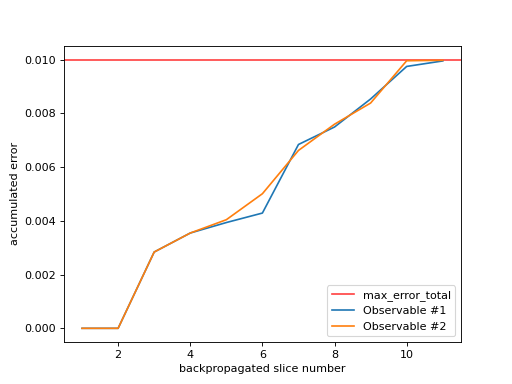
As you can see in the figure above, the number of backpropagated slices is displayed along the x-axis. You can think of this as the “time” of the backpropagation algorithm. The accumulated error due to truncated Pauli terms is displayed along the y-axis. If OBPMetadata.truncation_error_budget.max_error_total is not numpy.inf, it is displayed as a red horizontal line. Each observable that was backpropagated, gets its own line.

This data is related to the one visualized by plot_slice_errors(). This method plots the cumulative sum of the slice errors along the x-axis.

Parameters:

• metadata (OBPMetadata) – the metadata to be visualized.

• axes (Axes) – the matplotlib axes in which to plot.

Return type:

None

plot_left_over_error_budget(metadata, axes)

Plot the left-over error budget.

This method populates the provided figure axes with a line-plot of the OBPMetadata.left_over_error_budget(). Below is an example where we plot some metadata which exists within our context.

>>> from matplotlib import pyplot as plt
>>> from qiskit_addon_obp.utils.visualization import plot_left_over_error_budget
>>> fig, axes = plt.subplots(1, 1)
>>> plot_left_over_error_budget(metadata, axes)

(png, hires.png, pdf)

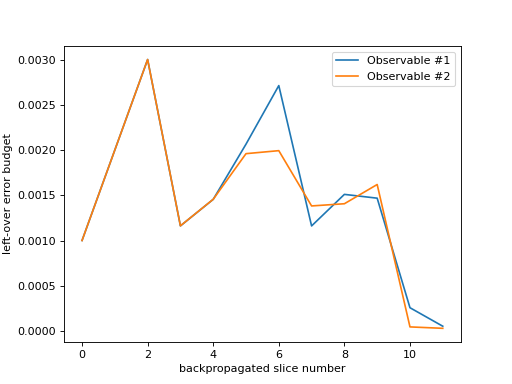
As you can see in the figure above, the number of backpropagated slices is displayed along the x-axis. You can think of this as the “time” of the backpropagation algorithm. The left-over error budget available at each backpropagation step is displayed along the y-axis. Since each observable that was backpropagated has its own budget, they are plotted as separate lines.

Parameters:

• metadata (OBPMetadata) – the metadata to be visualized.

• axes (Axes) – the matplotlib axes in which to plot.

Return type:

None

plot_slice_errors(metadata, axes)

Plot the slice errors.

This method populates the provided figure axes with a bar-plot of the truncation error incurred at each backpropagated slice. Below is an example where we plot some metadata which exists within our context.

>>> from matplotlib import pyplot as plt
>>> from qiskit_addon_obp.utils.visualization import plot_slice_errors
>>> fig, axes = plt.subplots(1, 1)
>>> plot_slice_errors(metadata, axes)

(png, hires.png, pdf)

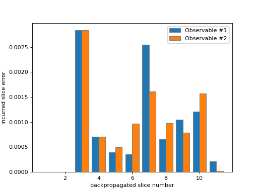
As you can see in the figure above, the number of backpropagated slices is displayed along the x-axis. You can think of this as the “time” of the backpropagation algorithm. The truncation error incurred at each backpropagation step is displayed along the y-axis. Since each observable is treated individually, they are plotted separately.

This data is related to the one visualized by plot_accumulated_error(). That method will plot the cumulative sum of the slice errors along the x-axis.

Parameters:

• metadata (OBPMetadata) – the metadata to be visualized.

• axes (Axes) – the matplotlib axes in which to plot.

Return type:

None

plot_num_paulis(metadata, axes)

Plot the number of Pauli terms.

This method populates the provided figure axes with a line-plot of the number of Pauli terms at each backpropagated slice. Below is an example where we plot some metadata which exists within our context.

>>> from matplotlib import pyplot as plt
>>> from qiskit_addon_obp.utils.visualization import plot_num_paulis
>>> fig, axes = plt.subplots(1, 1)
>>> plot_num_paulis(metadata, axes)

(png, hires.png, pdf)

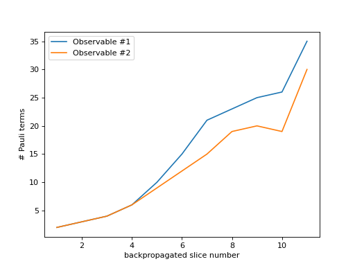
As you can see in the figure above, the number of backpropagated slices is displayed along the x-axis. You can think of this as the “time” of the backpropagation algorithm. The number of Pauli terms at each backpropagation step is displayed along the y-axis. Since each observable is treated individually, they are plotted separately.

You can also find out the number of unique Pauli terms across all observables by using plot_sum_paulis().

Parameters:

• metadata (OBPMetadata) – the metadata to be visualized.

• axes (Axes) – the matplotlib axes in which to plot.

Return type:

None

plot_num_truncated_paulis(metadata, axes)

Plot the number of truncated Pauli terms.

This method populates the provided figure axes with a bar-plot of the number of the truncated Pauli terms at each backpropagated slice. Below is an example where we plot some metadata which exists within our context.

>>> from matplotlib import pyplot as plt
>>> from qiskit_addon_obp.utils.visualization import plot_num_truncated_paulis
>>> fig, axes = plt.subplots(1, 1)
>>> plot_num_truncated_paulis(metadata, axes)

(png, hires.png, pdf)

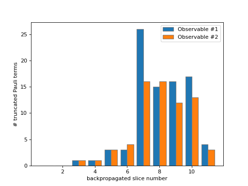
As you can see in the figure above, the number of backpropagated slices is displayed along the x-axis. You can think of this as the “time” of the backpropagation algorithm. The number of truncated Pauli terms at each backpropagation step is displayed along the y-axis. Since each observable is treated individually, they are plotted separately.

This data can give you additional insight as to how the accumulated error is split across multiple Pauli terms (see also the output of plot_accumulated_error()).

Parameters:

• metadata (OBPMetadata) – the metadata to be visualized.

• axes (Axes) – the matplotlib axes in which to plot.

Return type:

None

plot_sum_paulis(metadata, axes)

Plot the total number of all Pauli terms.

This method populates the provided figure axes with a line-plot of the total number of all Pauli terms at each backpropagated slice. Below is an example where we plot some metadata which exists within our context.

>>> from matplotlib import pyplot as plt
>>> from qiskit_addon_obp.utils.visualization import plot_sum_paulis
>>> fig, axes = plt.subplots(1, 1)
>>> plot_sum_paulis(metadata, axes)

(png, hires.png, pdf)

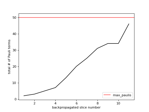
As you can see in the figure above, the number of backpropagated slices is displayed along the x-axis. You can think of this as the “time” of the backpropagation algorithm. The total number of all Pauli terms at each backpropagation step is displayed along the y-axis. If OBPMetadata.operator_budget.max_paulis is not None, it is displayed as a red horizontal line.

This data can give you additional insight into how many unique Pauli terms are spread across all of the backpropagated observables. See also the output of plot_num_paulis() for the number of Pauli terms in each observable individually.

Parameters:

• metadata (OBPMetadata) – the metadata to be visualized.

• axes (Axes) – the matplotlib axes in which to plot.

Return type:

None

plot_num_qwc_groups(metadata, axes)

Plot the number of qubit-wise commuting Pauli groups.

This method populates the provided figure axes with a line-plot of the number of qubit-wise commuting Pauli groups at each backpropagated slice. Below is an example where we plot some metadata which exists within our context.

>>> from matplotlib import pyplot as plt
>>> from qiskit_addon_obp.utils.visualization import plot_num_qwc_groups
>>> fig, axes = plt.subplots(1, 1)
>>> plot_num_qwc_groups(metadata, axes)

(png, hires.png, pdf)

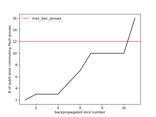
As you can see in the figure above, the number of backpropagated slices is displayed along the x-axis. You can think of this as the “time” of the backpropagation algorithm. The number of qubit-wise commuting Pauli groups at each backpropagation step is displayed along the y-axis. If OBPMetadata.operator_budget.max_qwc_groups is not None, it is displayed as a red horizontal line.

Parameters:

• metadata (OBPMetadata) – the metadata to be visualized.

• axes (Axes) – the matplotlib axes in which to plot.

Return type:

None