Tools to profile, customize, and inspect experiments
Usage estimate: 10 minutes on a Heron r2 processor (NOTE: This is an estimate only. Your runtime might vary.)
Getting good results from a quantum computer takes more than a well-designed circuit. The device's current condition, how your circuit is scheduled, the noise it experiences, and when and how your job runs on the quantum processing unit (QPU) all affect the quality of your results. Qiskit and IBM Quantum® Compute Service offer a growing set of developer tools that expose this information. You can use these tools to act on that information before you commit QPU time to a full experiment, and to debug a finished experiment.
This tutorial walks through a single end-to-end experiment and shows how to combine these tools at each stage of a typical development workflow. You refresh device properties to select a better layout, inspect circuit timing, learn a noise model and use it to preview the benefit of error mitigation with local simulation, estimate QPU usage, recalibrate readout at the start of a session, and finally inspect how your job ran on the hardware. Not every tool is useful for every experiment, so choose the tools that address the questions you have about your own workload.
The workflow is as follows:
- Prepare a mirror circuit of a Trotterized time evolution of a linear transverse-field Ising model.
- Select a backend with an alternative calibration data set designed for noise-model-based error mitigation methods.
- Run device benchmarking experiments so that the transpiler uses up-to-date device properties when selecting a layout.
- Inspect the timing information of the scheduled circuit.
- Learn Pauli-Lindblad and readout noise models for the circuit.
- Perform noiseless, unmitigated, and mitigated simulations by using the learned noise model. This shows how much improvement you might gain from the selected error mitigation methods: probabilistic error cancellation (PEC) and Twirled Readout Error eXtinction (TREX) in this tutorial.
- Get a usage estimate without QPU execution to see whether the experiment needs adjusting to fit your budget.
- Start a session and trigger calibration so that the experiment uses the most recent calibration data.
- Run the experiment on the QPU by using Estimator, and compare the hardware results with the simulated preview.
- Inspect the execution spans to see whether there are significant gaps between groups of executions (chunks).
Requirements
Before starting this tutorial, ensure that you have the following installed:
- Qiskit SDK v2.3 or later, with visualization support
qiskit-ibm-runtimev0.52 or later (pip install qiskit-ibm-runtime)- Qiskit Aer (
pip install qiskit-aer) - Plotly (
pip install plotly) - Qiskit Device Benchmarking (
pip install git+https://github.com/qiskit-community/qiskit-device-benchmarking.git)
Some steps in this tutorial are not available on every plan:
- Dry-run jobs (Steps 2.4 and 3.5) are available only on the Flex, Premium, and On-Prem plans.
- Sessions (Step 4.1) are not available on the Open Plan. To run in batch mode instead, set
run_calibration = Falsein Step 4.1.
Summary of tools used
Tool | What it tells you or does | Step | Docs |
|---|---|---|---|
| Specially calibrated instructions | Non-standard calibrations that can benefit some experiments. | 2.1 | Documentation |
| Qubit quality benchmarking | Refreshes device properties data. | 2.2 | Tutorial |
| Timing for scheduled circuits | Visualizes when each instruction runs, to help spot idle time and inefficient instruction alignment. | 2.4 | Documentation |
select-error-mitigation AI agent skill | Compares error mitigation methods for your workload and reports which ones to use and why. | 3.2 | GitHub repository |
| Client-side primitives | New implementations of the primitives that give more insight into, and control over, pre- and post-processing. | 3.2 | Documentation |
NoiseLearnerV3 | Performs noise learning using both the Pauli-Lindblad and TREX protocols. | 3.3 | Documentation |
| Local testing mode | Verifies syntactic correctness and compares the effects of different error mitigation methods. | 3.4 | Documentation |
| Usage estimation | Provides an accurate usage estimate before hardware execution. | 3.5 | Documentation |
| Calibration in sessions | Triggers calibration to ensure the experiment uses optimal readout parameters. | 4.1 | Documentation |
| Execution spans | Shows when each circuit configuration ran on the QPU, and in which order. | 4.4 | Documentation |
Step 1: Specify a circuit and observable
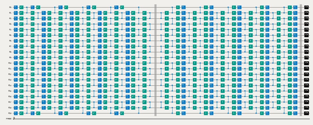
Prepare a mirror circuit of a Trotterized time evolution of a linear transverse-field Ising model. Mirror the circuit to cancel the circuit unitary and form an identity circuit. Because the ideal output is the all-zero state, the ideal expectation value of each single-qubit observable is 1. Mirroring also doubles the circuit depth, which amplifies the effect of noise.
import numpy as np
from qiskit.circuit import QuantumCircuit
from qiskit.quantum_info import SparsePauliOp


def construct_ising_circuit(
    num_qubits: int,
    num_trotter_steps: int,
    rx_angle: float,
    barrier: bool = True,
) -> QuantumCircuit:
    circuit = QuantumCircuit(num_qubits)

    for _step in range(num_trotter_steps):
        circuit.rx(rx_angle, range(num_qubits))
        if barrier:
            circuit.barrier()
        for first_qubit in (1, 2):
            for idx in range(first_qubit, num_qubits, 2):
                # equivalent to Rzz(-pi/2):
                circuit.sdg([idx - 1, idx])
                circuit.cz(idx - 1, idx)
        if barrier:
            circuit.barrier()

    return circuit


def mirror_circuit(circuit: QuantumCircuit) -> QuantumCircuit:
    mirror_circ = circuit.copy_empty_like()
    mirror_circ.compose(circuit, inplace=True)
    mirror_circ.barrier()
    mirror_circ.compose(circuit.inverse(), inplace=True)
    mirror_circ.measure_active()
    return mirror_circ
num_qubits = 20
observables = [
SparsePauliOp("I" * ((num_qubits - 1) - q) + "Z" + "I" * q)
for q in range(num_qubits)
]
# Free parameters of the demonstration circuit: the number of Trotter steps
# sets the circuit depth, and rx_angle is the transverse-field rotation angle
# applied in each step (pi/4 makes the dynamics non-Clifford)
num_trotter_steps = 5
rx_angle = np.pi / 4
circuit = construct_ising_circuit(
num_qubits, num_trotter_steps, rx_angle, barrier=False
)
mirrored_circuit = mirror_circuit(circuit)mirrored_circuit.draw(
"mpl", fold=-1, scale=0.3, idle_wires=False, measure_arrows=False
)Output:
Step 2: Optimize for quantum hardware execution
2.1 Use alternative calibration if applicable
IBM® QPUs are calibrated periodically for good performance across general use cases. Some workloads, however, benefit from instructions whose parameters are tuned differently. For more information, refer to Specially calibrated instructions.
This tutorial uses an alternative calibration data set called slow_gates_ac. This calibration contains a slower cz gate and modulates the two-level system (TLS) bias to stabilize device errors over time, which benefits error mitigation methods that rely on a learned noise model. The slow_gates_ac calibration is available only on Heron QPUs. Use slow_gates instead if you are running on a Nighthawk QPU.
from qiskit_ibm_runtime import QiskitRuntimeService

service = QiskitRuntimeService()
# Use slow_gates_ac because this tutorial uses a noise-learning-based mitigation method
backend = service.backend("ibm_kingston", calibration_id="slow_gates_ac")
2.2 Run real-time device benchmarking
One of the most critical stages of transpilation is layout selection, which maps virtual qubits in a circuit to physical qubits on the target device. A good layout minimizes the number of SWAP operations needed and places the circuit on the best-performing qubits, so the quality of the initial layout can significantly affect the quality of your results.
Periodic benchmarking routines run on every IBM QPU to report the current performance of its qubits: relaxation times (), coherence times (), readout errors, and one- and two-qubit gate errors. The Qiskit transpiler uses these metrics during layout selection.
Superconducting qubits, however, can drift on shorter timescales, and transient defects (known as two-level systems) can temporarily degrade a qubit that performed well at calibration time. The transpiler cannot pick the best layout if it is working from stale information, so it can be worth spending some QPU time characterizing the device before selecting a layout.
Refer to the Refresh backend properties with real-time benchmarking tutorial for a detailed walk-through.
The characterization suite builds several experiments, submits multiple jobs, and fits the results. This process can take a few minutes in total. Enable INFO-level logging so that each stage prints its progress as it runs.
import sys
import logging

logger = logging.getLogger("qiskit_device_benchmarking")
logger.setLevel(logging.INFO)
logger.addHandler(logging.StreamHandler(stream=sys.stdout))
BackendCharacterization is a convenience class that runs the characterization experiments of your choice, analyzes the results, and returns an updated Backend object that you can pass to the transpiler.
You might see a warning that a backend was passed in as the mode while a batch is open. This warning is expected, and you can safely ignore it.
from qiskit_ibm_runtime import Batch
from qiskit_device_benchmarking.utilities.characterization_utils import (
    BackendCharacterization,
)

# The full suite is ["readout", "rb_1q", "rb_2q", "t1", "t2"].
# Run a subset of the experiments to save time.
experiments = ["readout", "t1", "t2"]
characterizer = BackendCharacterization(backend)
with Batch(backend=backend):
    jobs = characterizer.run_experiments(experiments=experiments)
Output:
base_primitive.get_mode_service_backend:WARNING:2026-11-04 19:59:47,265: A backend was passed in as the mode but a session context manager is open so this job will run inside this session/batch instead of in job mode.
Building readout experiments
Building T1 experiments
Building T2 experiments
Readout job submitted: dblta1d8ft8s738tnpp0
T1 experiment submitted: ['dblta1t8ft8s738tnpq0']
T2 (Hahn) experiment submitted: ['dblta2hkbkrc73cocepg']
# Retrieve all job results and update the backend data
characterizer.analyze_results()
backend_updated = characterizer.update_backend()
Output:
Updating readout error
Updating T1
Updating T2
2.3 Transpile to ISA
Transform the circuit and observables to match the backend's instruction set architecture (ISA) by using the refreshed device properties.
from qiskit.transpiler.preset_passmanagers import generate_preset_pass_manager

pm = generate_preset_pass_manager(
    backend=backend_updated, optimization_level=3
)
isa_circuit = pm.run(mirrored_circuit)
isa_observables = [
    observable.apply_layout(isa_circuit.layout) for observable in observables
]
2.4 Visualize circuit timing
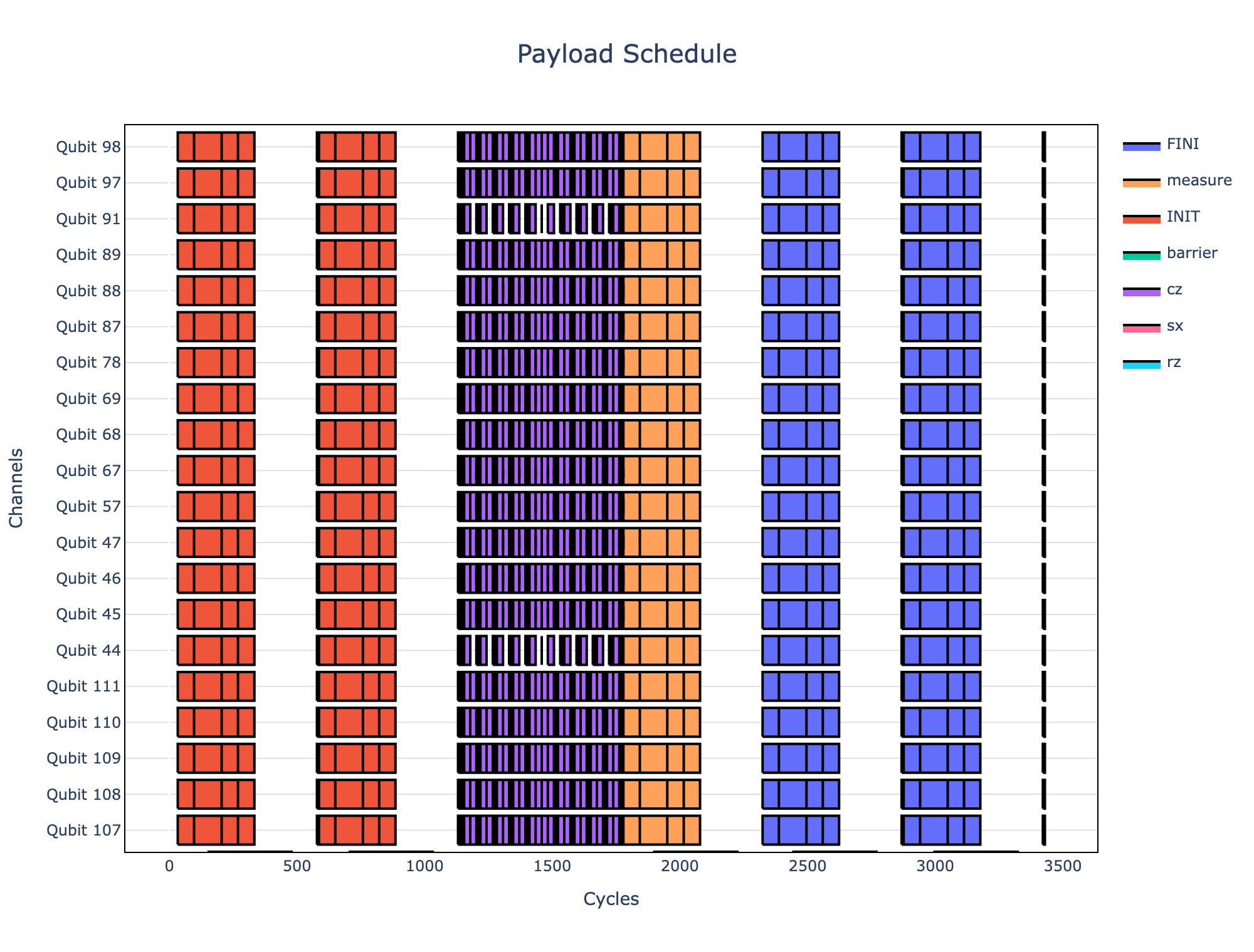
In addition to visualizing instructions on a circuit, you might want to visualize a circuit's scheduling to quickly spot idle time on qubits or inefficient instruction alignment. You can get the most detailed and accurate timing information from IBM Quantum Compute Service by using dry-run mode.
The circuit in this tutorial is static, so its schedule is not very informative. You could get similar timing information locally from the circuit and the backend properties, for example by using the timeline drawer built in to Qiskit. This step is included to show how to request and visualize the timing information. The service-provided timing is most useful for dynamic circuits. Dynamic circuits contain mid-circuit measurements, conditional operations, and feedforward, which add implicit operations such as broadcasting measurement results and determining branches. The timing of these operations cannot be determined from the circuit and backend properties alone.
Refer to Visualize circuit timing for more information.
Scheduled circuit timing is available only for Sampler and Executor jobs, so the following cell submits the circuit in dry-run mode by using Sampler. Jobs submitted in dry-run mode do not run on real QPUs and are not charged.
from qiskit_ibm_runtime.executor_sampler import Sampler

sampler = Sampler(backend)
# Request timing information in the result metadata
sampler.options.experimental = {
    "execution": {
        "scheduler_timing": True,
    },
}

# Specify dry_run=True to submit in dry-run mode
sampler_job = sampler.run([isa_circuit], dry_run=True)
job_result = sampler_job.result()
circuit_schedule = job_result[0].metadata["compilation"]["scheduler_timing"]
circuit_schedule_timing = circuit_schedule["timing"]from qiskit_ibm_runtime.visualization import draw_circuit_schedule_timing
# Create a figure from the metadata
fig = draw_circuit_schedule_timing(
circuit_schedule=circuit_schedule_timing,
included_channels=None,
filter_readout_channels=False,
filter_barriers=False,
width=1000,
)
# For large circuits, displaying the figure inline can hang your Jupyter session.
# Uncomment the following to save it to an HTML file instead.
# fig.write_html("scheduler_timing.html")
# For small circuits, uncomment the following line to display the figure inline.
# fig.show(renderer="notebook")This figure is too large to display in a notebook. The following screenshot shows a summarized view.
Step 3: Apply error mitigation and test locally
3.1 Cliffordize the circuit
The cost of general noisy simulation grows exponentially with the number of qubits, and most laptops cannot simulate more than about 32 qubits. Therefore, first convert the circuit to a Clifford circuit, which a stabilizer simulator can handle far more efficiently. The conversion rounds each rotation angle to a Clifford angle, so the simulated circuit approximates the original circuit rather than reproducing it.
from qiskit.transpiler import PassManager
from qiskit_ibm_runtime.transpiler.passes import ConvertISAToClifford

clifford_circuit = PassManager([ConvertISAToClifford()]).run(isa_circuit)
clifford_pubs = [(clifford_circuit, isa_observables)]
3.2 Apply PEC with TREX
Selecting error mitigation methods that balance cost and accuracy for your specific experiment can be difficult. You can use the select-error-mitigation AI agent skill to analyze the available methods for your workload. The skill presents a summary report that explains whether each method was selected and why.
Refer to the Qiskit AI skills GitHub repository for more information.
This tutorial uses PEC with TREX directly, so that you can follow along without an AI agent.
PEC is a technique for mitigating quantum noise in observable expectation value calculations. Under ideal conditions, it can produce an unbiased estimate of the expectation values by learning the noise of each layer of two-qubit gates, then executing an ensemble of circuits that, on average, apply the inverse of that noise. Pauli twirling is used to tailor the noise into a Pauli channel so that it can be learned and inverted efficiently.
In practice, PEC is only as accurate as the learned noise model. The sparse Pauli-Lindblad model includes only one- and two-qubit error terms on neighboring qubits, and it cannot fully capture effects such as crosstalk between distant qubits or time-correlated errors. The device noise can also drift between noise learning and execution. Any noise that the model misses is not canceled, and any noise that the model overestimates is overcompensated, so mitigated results can still deviate from the ideal values in either direction.
TREX is a technique that mitigates measurement errors and is useful for estimating Pauli observable expectation values. It relies on measurement twirling, which diagonalizes the readout-error transfer matrix and makes it easy to invert. A rescaling term is learned from the diagonal noise channel by measuring twirled calibration circuits that are initialized in the zero state.
You can enable both PEC and TREX through Estimator options. This tutorial uses the client-side implementations of the Qiskit SamplerV2 and EstimatorV2 interfaces, introduced in qiskit-ibm-runtime v0.50.0. These client-side primitives perform most of the pre- and post-processing locally and delegate execution to the Executor primitive. Running on the client side provides greater transparency, faster debugging feedback, and finer control.
Because they implement the same API, the client-side primitives are largely drop-in replacements for the legacy server-side primitives; usually the only change needed is the import statement.
Enable INFO-level logging to see the progress of client-side pre- and post-processing.
import logging

logger = logging.getLogger("qiskit_ibm_runtime")
logger.setLevel(logging.INFO)
from qiskit_ibm_runtime.executor_estimator import Estimator
estimator = Estimator(mode=backend)# Enable TREX
estimator.options.resilience.measure_mitigation = True
# Enable PEC
estimator.options.resilience.pec_mitigation = True3.3 Learn noise models and run Cliffordized circuit
Both PEC and TREX require noise learning, which you can do with NoiseLearnerV3. The steps are as follows:
- Find the unique two-qubit gate layers and measurement layers in the circuit, for the Pauli-Lindblad and TREX protocols, respectively.
- Pass the layers to
NoiseLearnerV3to learn the noise models. - Convert the learned noise models to Pauli-Lindblad maps.
Estimator doesn't use a pre-learned TREX noise model, but you can still use the learned readout model in the noisy simulation.
Refer to Noise learning helper for more information about NoiseLearnerV3.
In addition to running the noise-learning experiment, you also run the Cliffordized circuit on the QPU. This step is not always necessary, but it is useful for comparing against the simulated results in a later step. Run both in a batch to minimize how much the noise profile drifts between the two.
pubs = [(isa_circuit, isa_observables)]
# Specify types="all" to find layers for both Pauli-Lindblad and TREX learning
layers = estimator.find_unique_layers(pubs, types="all")
print(f"Number of unique layers found: {len(layers)}")
Output:
Number of unique layers found: 3
from qiskit_ibm_runtime import NoiseLearnerV3

with Batch(backend) as batch:
    learner = NoiseLearnerV3(batch)
    learner.options.num_randomizations = 64
    learner.options.shots_per_randomization = 128
    learner.options.environment.job_tags = [
        "noise-learning",
        f"{len(layers)} layers",
    ]
    learner_job = learner.run(layers)
    print(f"NoiseLearner job id: {learner_job.job_id()}")

    clifford_estimator = Estimator(batch)
    clifford_estimator.options.environment.job_tags = [
        "cliffordized",
        "unmitigated",
    ]
    clifford_estimator.options.resilience.measure_mitigation = False
    clifford_estimator.options.twirling.enable_measure = True
    clifford_estimator.options.twirling.enable_gates = True

    clifford_job = clifford_estimator.run(clifford_pubs)
    print(f"Clifford job id: {clifford_job.job_id()}")
Output:
runtime.program_run:INFO:2026-11-04 20:18:59,955: Posting the API request.
runtime.program_run:INFO:2026-11-04 20:19:00,467: Payload size: 0 MB.
estimator.run:INFO:2026-11-04 20:19:00,468: Starting pre-processing
prepare._build_quantum_program:INFO:2026-11-04 20:19:00,471: Processing pub 1/1 with MitigationTask.
estimator.run:INFO:2026-11-04 20:19:00,577: Submitting 1 pub to executor with 4096 total shots
NoiseLearner job id: dbltj158ft8s738tochg
runtime.program_run:INFO:2026-11-04 20:19:01,207: Posting the API request.
runtime.program_run:INFO:2026-11-04 20:19:02,108: Payload size: 0 MB.
Clifford job id: dbltj19kbkrc73cod180
learner_result = learner_job.result()
pauli_lindblad_maps = learner_result.to_pauli_lindblad_maps()
clifford_result = clifford_job.result()
print(">>> Expectation values from unmitigated Clifford circuit:")
print(clifford_result[0].data.evs)Output:
>>> Expectation values from unmitigated Clifford circuit:
[0.80371094 0.76708984 0.73095703 0.72119141 0.66210938 0.66552734
 0.61962891 0.65283203 0.6328125  0.640625   0.64599609 0.67138672
 0.62988281 0.64648438 0.61572266 0.63330078 0.61865234 0.69091797
 0.71337891 0.76171875]
3.4 Perform local simulation
With qiskit-ibm-runtime local testing mode, you can perform both noiseless and noisy simulations locally with minimal code changes. This is useful for verifying syntactic correctness, comparing the effects of different mitigation methods, and checking how well the learned noise model agrees with hardware results.
Local mode is designed to share largely the same interface as the QPU execution path. In most cases, you only need to change the backend passed when initializing the primitive and rerun the same code. Each of the following subsections creates its own Estimator instance, so you can run them without going back and changing a previous cell.
Refer to Local testing mode for more information.
3.4.1 Run a noiseless simulation
from qiskit_aer import AerSimulator

sim_estimator = Estimator(AerSimulator(method="stabilizer"))
sim_estimator.options.resilience_level = 0
sim_estimator_job = sim_estimator.run(clifford_pubs)
ideal_result = sim_estimator_job.result()
print(">>> Ideal expectation values from simulation:")
print(ideal_result[0].data.evs)
Output:
>>> Ideal expectation values from simulation:
[1. 1. 1. 1. 1. 1. 1. 1. 1. 1. 1. 1. 1. 1. 1. 1. 1. 1. 1. 1.]
3.4.2 Run a noisy simulation with the learned Pauli-Lindblad model
Do not use a fake backend or a Qiskit Aer noise model if you plan to use the learned Pauli-Lindblad noise model in your local simulation. Otherwise, the simulation applies the noise twice.
sim_estimator_noisy = Estimator(AerSimulator(method="stabilizer"))
sim_estimator_noisy.options.resilience_level = 0
# Twirling is required for find_unique_layers to work
sim_estimator_noisy.options.twirling.enable_gates = True
sim_estimator_noisy.options.twirling.enable_measure = True
clifford_layers = sim_estimator_noisy.find_unique_layers(
    clifford_pubs, types="all"
)
# Pass noise model for both 2Q and measurement layers for noisy simulation.
sim_estimator_noisy.options.simulator.layer_noise_model = zip(
    clifford_layers, pauli_lindblad_maps
)
sim_estimator_noisy_job = sim_estimator_noisy.run(clifford_pubs)
sim_noisy_result = sim_estimator_noisy_job.result()
print(">>> Unmitigated expectation values from simulation:")
print(sim_noisy_result[0].data.evs)Output:
>>> Unmitigated expectation values from simulation:
[0.85449219 0.8203125  0.75634766 0.76025391 0.67578125 0.703125
 0.66308594 0.70800781 0.66699219 0.69335938 0.74658203 0.76464844
 0.72753906 0.74853516 0.74951172 0.734375   0.73144531 0.77929688
 0.79150391 0.83886719]
3.4.3 Run a noisy simulation with PEC and TREX
sim_estimator_mitigated = Estimator(AerSimulator(method="stabilizer"))

# Twirling is required for find_unique_layers to work
sim_estimator_mitigated.options.twirling.enable_gates = True
sim_estimator_mitigated.options.twirling.enable_measure = True

# Enable PEC & TREX
sim_estimator_mitigated.options.resilience.pec_mitigation = True
sim_estimator_mitigated.options.resilience.measure_mitigation = True

clifford_layers = sim_estimator_mitigated.find_unique_layers(
    clifford_pubs, types="all"
)

# This sets the noise model
sim_estimator_mitigated.options.simulator.layer_noise_model = zip(
    clifford_layers, pauli_lindblad_maps
)
# This tells PEC which noise to cancel
sim_estimator_mitigated.options.resilience.layer_noise_model = zip(
    clifford_layers, pauli_lindblad_maps
)
sim_estimator_mitigated_job = sim_estimator_mitigated.run(clifford_pubs)
sim_mitigated_result = sim_estimator_mitigated_job.result()
print(">>> Mitigated expectation values from simulation:")
print(sim_mitigated_result[0].data.evs)Output:
>>> Mitigated expectation values from simulation:
[0.97875512 1.06589736 0.98762488 1.06136389 0.98047201 0.95644499
 0.91897594 0.94272622 0.97158012 0.93390746 1.02496886 0.87936432
 1.07405883 0.94506833 1.07373448 0.96440822 0.99443521 1.01167907
 0.87564838 0.94097861]
3.4.4 Compare the simulation results
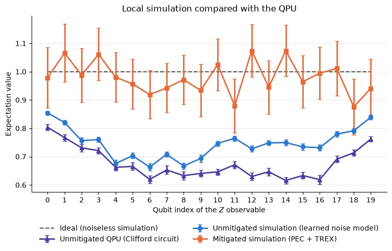
Plot the expectation value of each single-qubit observable from the three simulations, together with the unmitigated QPU result for the same Clifford circuit from Step 3.3. Because the circuit is a mirror circuit, every ideal value is 1. The error bars show the standard error that Estimator reports for each value.
The closer the unmitigated simulation is to the unmitigated QPU result, the better the learned noise model describes the hardware. Compare the shapes of the two curves as well as the gap between them. If the curves have a similar shape but are offset, the model captures how the noise is distributed across qubits but underestimates or overestimates its overall strength. Errors in specific qubits or layers show up as qubits that deviate from the common shape.
Use this comparison as a check before you spend QPU time on the mitigated experiment: if the two disagree significantly, PEC is unlikely to get close to the ideal values on hardware either. In that case, relearning the noise model or selecting a different layout is a better next step than running more shots. You can also relearn the noise model with different NoiseLearnerV3 options, such as more randomizations or additional layer-pair depths, and check whether the agreement improves. For example, this tutorial sets num_randomizations to 64 instead of the default of 32 in Step 3.3, because the additional randomizations improved the agreement for this circuit. NoiseLearnerV3 runs a standard learning protocol. For full control over the learning experiment, you can build your own with Qiskit noise learning.
import matplotlib.pyplot as plt

qubit_indices = np.arange(num_qubits)
results_to_plot = {
    "Unmitigated QPU (Clifford circuit)": (clifford_result, "#4a3aa7", "^"),
    "Unmitigated simulation (learned noise model)": (
        sim_noisy_result,
        "#2a78d6",
        "o",
    ),
    "Mitigated simulation (PEC + TREX)": (
        sim_mitigated_result,
        "#eb6834",
        "s",
    ),
}

fig, ax = plt.subplots(figsize=(9, 4.5))
ax.plot(
    qubit_indices,
    ideal_result[0].data.evs,
    color="#52514e",
    linestyle="--",
    linewidth=1.5,
    label="Ideal (noiseless simulation)",
)
for label, (result, color, marker) in results_to_plot.items():
    ax.errorbar(
        qubit_indices,
        result[0].data.evs,
        yerr=result[0].data.stds,
        color=color,
        marker=marker,
        markersize=6,
        linewidth=2,
        capsize=3,
        label=label,
    )

ax.set_xlabel("Qubit index of the $Z$ observable")
ax.set_ylabel("Expectation value")
ax.set_title("Local simulation compared with the QPU")
ax.set_xticks(qubit_indices)
ax.grid(axis="y", alpha=0.3)
ax.spines[["top", "right"]].set_visible(False)
# Place the legend below the plot so it doesn't cover any data
ax.legend(
    frameon=False, loc="upper center", bbox_to_anchor=(0.5, -0.15), ncol=2
)
plt.show()
Output:
3.5 Estimate usage
The main use case of dry-run mode is usage estimation. Unlike local execution mode, dry-run mode submits the job to IBM Quantum Compute Service, which returns an accurate usage estimate but random result data. Dry-run jobs do not run on real QPUs and do not consume any QPU time.
Dry-run jobs are not available on the Open or Pay-As-You-Go plans.
Refer to Dry-run jobs for more information.
import time

dry_run_estimator = Estimator(mode=backend)
dry_run_estimator.options.resilience.measure_mitigation = True
dry_run_estimator.options.resilience.pec_mitigation = True
dry_run_estimator.options.resilience.layer_noise_model = zip(
    layers, pauli_lindblad_maps
)

dry_run_job = dry_run_estimator.run(
    [(isa_circuit, isa_observables)], dry_run=True
)
# Wait for the job to finish to get an accurate estimate
dry_run_job.result()
# Sometimes it takes a second for usage to get updated
time.sleep(1)
print(f">>> Usage is {dry_run_job.usage()} seconds")
Output:
estimator.run:INFO:2026-11-04 20:54:52,151: Starting pre-processing
prepare._build_quantum_program:INFO:2026-11-04 20:54:52,161: Processing pub 1/1 with PEC.
trex.apply_trex:INFO:2026-11-04 20:54:52,295: TREX calibration circuit added (64 randomizations).
estimator.run:INFO:2026-11-04 20:54:52,295: Submitting 2 pubs to executor with 133696 total shots
runtime.program_run:INFO:2026-11-04 20:54:53,210: Posting the API request.
runtime.program_run:INFO:2026-11-04 20:54:53,795: Payload size: 0 MB.
post_processor_v0_1.estimator_v2_post_processor_v0_1:INFO:2026-11-04 20:55:09,906: Post-processing pub 1/1 (PEC).
>>> Usage is 42 seconds
Step 4: Run on hardware
4.1 Initialize a session and run calibration
Calibrating a QPU requires optimizing many parameters that define the electrical signals driving the quantum gates and operations. Calibration jobs run throughout the day in between user jobs, but not during an active session. Because these parameters can drift within a short period of time, it might be worth triggering calibration at the start of a session, or periodically during a long-running session, if you want the best possible results.
Currently, only readout calibration is supported, and it takes approximately five minutes of wall-clock time.
from qiskit_ibm_runtime import Session, Batch, Calibrator

# Set to False to skip the session and calibration and run in batch mode instead
run_calibration = False
mode = Session(backend) if run_calibration else Batch(backend)

if run_calibration:
    calibrator = Calibrator(mode)
    # Wait for calibration to finish before submitting the experiment.
    calibrator.run().result()
4.2 Run on hardware with Estimator
The following cells run three jobs in the batch or session:
- A noise-learning experiment to refresh the noise model. This is useful if you expect the noise model from Step 3.3 to be stale by the time the Estimator job runs. In a batch, the Estimator jobs can run much later than the noise-learning job, because jobs from other users can run on the QPU in between. A session gives your workload exclusive access to the QPU, so the noise model is more likely to still be accurate when the experiment runs.
- The experiment with mitigation.
- The experiment without mitigation, for comparison.
learner = NoiseLearnerV3(mode)
learner.options.num_randomizations = 64
learner.options.shots_per_randomization = 128
learner_job = learner.run(layers)
print(f"NoiseLearner job id: {learner_job.job_id()}")
learner_result = learner_job.result()
pauli_lindblad_maps = learner_result.to_pauli_lindblad_maps()
Output:
NoiseLearner job id: dbmu831kbkrc73cq6m20
mitigated_estimator = Estimator(mode)
mitigated_estimator.options.environment.job_tags = ["pec", "trex"]
mitigated_estimator.options.resilience.measure_mitigation = True
mitigated_estimator.options.resilience.pec_mitigation = True
# Pass the learned noise model for PEC.
# PEC doesn't apply mitigation to the measurement layer and will simply ignore it.
mitigated_estimator.options.resilience.layer_noise_model = zip(
    layers, pauli_lindblad_maps
)

mitigated_job = mitigated_estimator.run([(isa_circuit, isa_observables)])
print(f">>> Mitigated job id: {mitigated_job.job_id()}")

unmitigated_estimator = Estimator(mode)
unmitigated_estimator.options.resilience_level = 0
unmitigated_estimator.options.environment.job_tags = ["unmitigated"]
unmitigated_job = unmitigated_estimator.run([(isa_circuit, isa_observables)])
print(f">>> Unmitigated job id: {unmitigated_job.job_id()}")

# Don't forget to close the session or batch if you're using one!
mode.close()
Output:
estimator.run:INFO:2026-11-04 20:55:24,399: Starting pre-processing
prepare._build_quantum_program:INFO:2026-11-04 20:55:24,405: Processing pub 1/1 with PEC.
trex.apply_trex:INFO:2026-11-04 20:55:24,572: TREX calibration circuit added (64 randomizations).
estimator.run:INFO:2026-11-04 20:55:24,572: Submitting 2 pubs to executor with 133696 total shots
runtime.program_run:INFO:2026-11-04 20:55:25,416: Posting the API request.
runtime.program_run:INFO:2026-11-04 20:55:26,089: Payload size: 0 MB.
estimator.run:INFO:2026-11-04 20:55:26,091: Starting pre-processing
prepare._build_quantum_program:INFO:2026-11-04 20:55:26,094: Processing pub 1/1 with MitigationTask.
estimator.run:INFO:2026-11-04 20:55:26,150: Submitting 1 pub to executor with 4096 total shots
>>> Mitigated job id: dblu43d8mdtc73d6s27g
runtime.program_run:INFO:2026-11-04 20:55:26,973: Posting the API request.
runtime.program_run:INFO:2026-11-04 20:55:27,480: Payload size: 0 MB.
>>> Unmitigated job id: dblu43u74qds73dr6c50
mitigated_result = mitigated_job.result()
print(">>> Expectation values from mitigated QPU run:")
print(mitigated_result[0].data.evs)
Output:
>>> Expectation values from mitigated QPU run:
[1.0406517  1.00620641 0.9724645  0.97155332 1.04062137 1.03094335
 0.99566392 0.98223681 1.01879461 1.06673953 1.06054294 1.07235231
 1.04693515 1.04113397 1.00350255 0.97067178 1.00089054 1.02635426
 1.05299946 1.0819404 ]
unmitigated_result = unmitigated_job.result()
print(">>> Expectation values from unmitigated QPU run:")
print(unmitigated_result[0].data.evs)
Output:
>>> Expectation values from unmitigated QPU run:
[0.953125   0.90771484 0.87744141 0.82324219 0.6796875  0.75097656
 0.69335938 0.82861328 0.83300781 0.86279297 0.88720703 0.86914062
 0.75439453 0.74658203 0.68115234 0.74707031 0.72558594 0.86035156
 0.91259766 0.92871094]
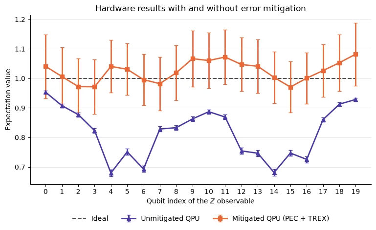
Plot the mitigated and unmitigated hardware results together with the ideal values. Because the circuit is a mirror circuit, every ideal value is 1, so the distance between each point and the dashed line shows the remaining error. Any remaining deviation from the ideal value, whether above or below it, reflects the statistical uncertainty of PEC and the limits of the learned noise model described in Step 3.2.
To further improve the results, you can try the following:
- Increase the number of shots or randomizations to reduce the statistical uncertainty of the mitigated estimates. The cost grows with the PEC sampling overhead.
- Relearn the noise model immediately before the experiment, in the same session, to reduce the effect of noise drift.
- Learn the noise model more precisely by increasing the
num_randomizations,shots_per_randomization, orlayer_pair_depthsoptions ofNoiseLearnerV3. Errors in the learned rates bias the mitigated results, and running more PEC shots does not remove this bias. - Add non-Markovian error checks to detect shots that are likely corrupted by non-Markovian errors, which the learned noise model does not describe, and discard them by postselection. Apply the same checks when you learn the noise model, by using the
bit_flip_checksoptions ofNoiseLearnerV3. Otherwise, the learned model includes errors that postselection removes from the experiment, and PEC overcompensates for them. Stricter postselection discards more shots, so balance the accuracy gain against the number of shots kept.
import matplotlib.pyplot as plt

qubit_indices = np.arange(num_qubits)
# The mirror circuit is an identity circuit, so every ideal value is 1
ideal_evs = np.ones(num_qubits)
results_to_plot = {
    "Unmitigated QPU": (unmitigated_result, "#4a3aa7", "^"),
    "Mitigated QPU (PEC + TREX)": (mitigated_result, "#eb6834", "s"),
}

fig, ax = plt.subplots(figsize=(9, 4.5))
ax.plot(
    qubit_indices,
    ideal_evs,
    color="#52514e",
    linestyle="--",
    linewidth=1.5,
    label="Ideal",
)
for label, (result, color, marker) in results_to_plot.items():
    ax.errorbar(
        qubit_indices,
        result[0].data.evs,
        yerr=result[0].data.stds,
        color=color,
        marker=marker,
        markersize=6,
        linewidth=2,
        capsize=3,
        label=label,
    )

ax.set_xlabel("Qubit index of the $Z$ observable")
ax.set_ylabel("Expectation value")
ax.set_title("Hardware results with and without error mitigation")
ax.set_xticks(qubit_indices)
ax.grid(axis="y", alpha=0.3)
ax.spines[["top", "right"]].set_visible(False)
# Place the legend below the plot so it doesn't cover any data
ax.legend(
    frameon=False, loc="upper center", bbox_to_anchor=(0.5, -0.15), ncol=3
)
plt.show()
Output:
4.3 Compare hardware and simulation results
Step 3.4 used local simulation to preview how much PEC and TREX would improve the results. Compare that preview with what the QPU delivered. If the simulated improvement and the hardware improvement are similar, local simulation is a useful way to evaluate mitigation settings for this workload before you spend QPU time on them.
The comparison is approximate, for three reasons:
- The simulations run the Cliffordized circuit from Step 3.1, while the hardware jobs run the original circuit.
- The simulations use the noise model learned in Step 3.3, while the mitigated hardware job uses the noise model that was refreshed in Step 4.2.
- The unmitigated hardware job uses resilience level 0, which disables twirling, while the unmitigated simulation uses twirling.
For a like-for-like check of the noise model itself, use the comparison of the Clifford circuit in Step 3.4.4.
fig, axes = plt.subplots(1, 2, figsize=(12, 4.5), sharey=True)
panels = {
    "Local simulation (Clifford circuit)": {
        "Unmitigated": (sim_noisy_result, "#2a78d6", "o"),
        "Mitigated (PEC + TREX)": (sim_mitigated_result, "#eb6834", "s"),
    },
    "QPU (original circuit)": {
        "Unmitigated": (unmitigated_result, "#4a3aa7", "^"),
        "Mitigated (PEC + TREX)": (mitigated_result, "#eb6834", "s"),
    },
}

for ax, (title, results_to_plot) in zip(axes, panels.items()):
    ax.axhline(
        1, color="#52514e", linestyle="--", linewidth=1.5, label="Ideal"
    )
    for label, (result, color, marker) in results_to_plot.items():
        ax.errorbar(
            qubit_indices,
            result[0].data.evs,
            yerr=result[0].data.stds,
            color=color,
            marker=marker,
            markersize=5,
            linewidth=2,
            capsize=3,
            label=label,
        )
    ax.set_title(title)
    ax.set_xlabel("Qubit index of the $Z$ observable")
    ax.set_xticks(qubit_indices[::2])
    ax.grid(axis="y", alpha=0.3)
    ax.spines[["top", "right"]].set_visible(False)
    # Place the legend below the plot so it doesn't cover any data
    ax.legend(
        frameon=False, loc="upper center", bbox_to_anchor=(0.5, -0.15), ncol=3
    )

axes[0].set_ylabel("Expectation value")
plt.tight_layout()
plt.show()

# Summarize each result by its mean absolute deviation from the ideal value of 1
for title, results_to_plot in panels.items():
    for label, (result, _, _) in results_to_plot.items():
        error = np.mean(np.abs(result[0].data.evs - 1))
        print(f"{title:<36} {label:<24} mean absolute deviation: {error:.3f}")
Output:
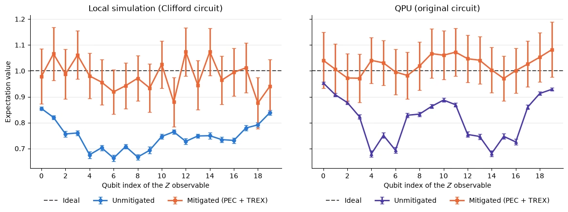
Local simulation (Clifford circuit)  Unmitigated              mean absolute deviation: 0.254
Local simulation (Clifford circuit)  Mitigated (PEC + TREX)   mean absolute deviation: 0.052
QPU (original circuit)               Unmitigated              mean absolute deviation: 0.184
QPU (original circuit)               Mitigated (PEC + TREX)   mean absolute deviation: 0.035
In this run, mitigation reduced the mean absolute deviation by about a factor of five both in the simulation and on the QPU, and the mitigated values agree with 1 within their error bars.
4.4 Inspect execution spans
When you submit circuits with multiple configurations, such as with gate twirling, IBM Quantum Compute Service does not necessarily execute all circuit configurations at once. Instead, it groups them into chunks and executes one chunk per shot loop. A shot loop is a single round of execution on the quantum hardware, in which every circuit in the chunk is run for the requested number of shots.
All jobs submitted to a real QPU go through some classical pre-processing, such as translation into pulses that can be sent to the hardware. Because this pre-processing can be done in parallel, the service dequeues and starts multiple jobs at a time. The QPU, however, can only process one unit of work at a time. This means that if your job generates multiple chunks, its chunks might be interleaved with those of other users' jobs, and each chunk might have to wait for its turn on the QPU.
QPU execution timing data for each chunk is reported in the job result metadata. The following visualization shows whether there are significant gaps between the executions of the chunks in your job. If the gaps are wider than your experiment can tolerate, you might want to rerun the job, or use session execution mode, which gives your workload exclusive access to the QPU.
Refer to View execution spans for more information.
chunk_timing = mitigated_result.metadata["executor"].chunk_timing

print(f"{len(chunk_timing)} chunks were executed.")
chunk_1 = chunk_timing[0]
print(f"The first chunk contains {len(chunk_1.parts)} parts.")
for idx, part in enumerate(chunk_1.parts):
    print(
        f"    Part {idx} contains {part.size} configurations from circuit {part.idx_item}"
    )
Output:
3 chunks were executed.
The first chunk contains 2 parts.
    Part 0 contains 103 configurations from circuit 0
    Part 1 contains 2 configurations from circuit 1
from qiskit_ibm_runtime.visualization import draw_chunk_timings

draw_chunk_timings(chunk_timing)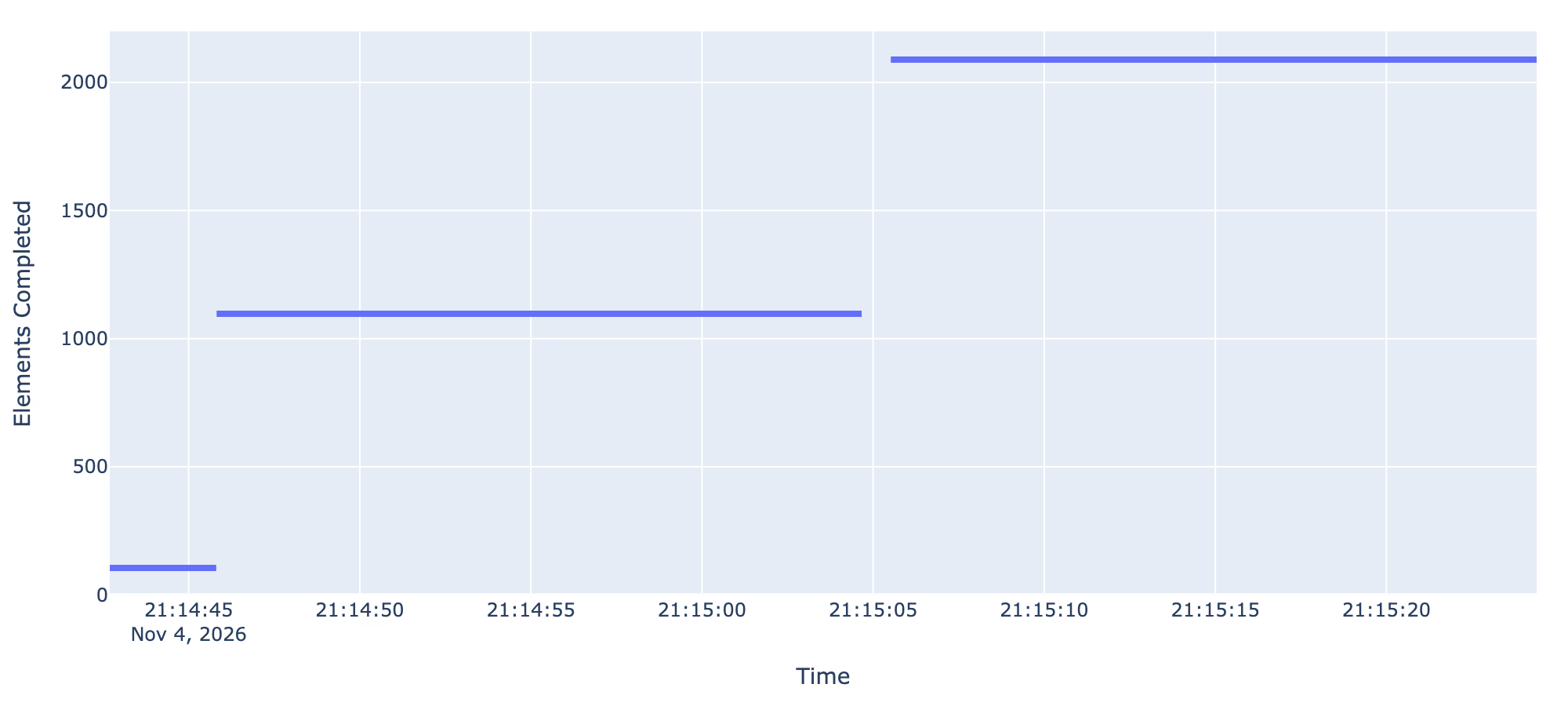
Next steps
- Rerun the experiment with and without the refreshed device properties (Step 2.2), the
slow_gates_accalibration (Step 2.1), or session calibration (Step 4.1) to measure how much each tool contributes for your workload. - Try a cheaper error mitigation method such as zero-noise extrapolation (ZNE), and use local simulation and dry-run usage estimates to compare its cost and accuracy against PEC. The
select-error-mitigationAI agent skill can help guide this choice. - Explore the full characterization suite, including randomized benchmarking, in the Refresh backend properties with real-time benchmarking tutorial.
- Learn more about the client-side primitives and the Executor in Migrate to client-side primitives.
- Apply these tools to your own experiments, starting with the ones that address your biggest source of uncertainty, whether that is device quality, noise, cost, or execution timing.