Simulate neutron scattering with an AQC + Trotter dynamics Serverless workflow
Usage estimate: 18 minutes on a Heron r3 processor (NOTE: This is an estimate only. Your runtime might vary.)
Learning outcomes
After completing this tutorial, you can expect to understand:
- How an inelastic neutron-scattering spectrum maps to the dynamical structure factor of a 1D quantum magnet.
- How to prepare the KCuF (isotropic Heisenberg) ground state with the density matrix renormalization group (DMRG) and matrix product state (MPS) fidelity maximization.
- How to run Trotter time-evolution, approximate quantum compilation (AQC) circuit compression, and mitigated execution as a single function call.
- How to post-process the per-site time series into and identify the two-spinon continuum.
Prerequisites
- Familiarity with Qiskit Patterns,
SparsePauliOp, and Trotter time-evolution. - Basic exposure to tensor-network methods (DMRG and MPS) is helpful but not required, as is familiarity with the
qiskit-addon-aqc-tensorlibrary that the function uses to compress Trotter circuits.
Background
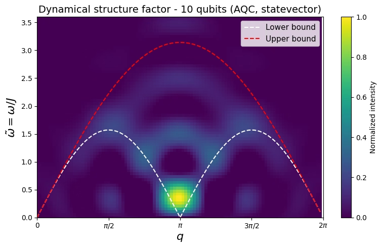
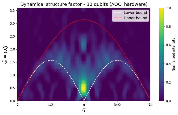
Inelastic neutron scattering measures the dynamical structure factor , the space-and-time Fourier transform of the spin-spin correlation function, so reproducing from a microscopic spin model is a direct, falsifiable test of a quantum simulation. This tutorial studies KCuF, a spin- antiferromagnetic Heisenberg chain whose excitations are not single spin flips but pairs of fractionalized spinons: instead of a sharp magnon dispersion, shows a broad two-spinon continuum, bounded below by and above by . Those are the dashed curves on the plots below. The physics in full, and the comparison against measured neutron data, are covered in the original tutorial and in Lee et al., arXiv:2603.15608.
The quantum workflow mirrors the scattering experiment:
- Prepare the chain's ground state .
- Kick it with a local perturbation at the center site, a -rotation, mimicking the momentum and energy transfer from the neutron.
- Time-evolve under the Heisenberg Hamiltonian, , with a Trotter product formula.
- Measure the per-site magnetization ; as a function of site and time this is the retarded Green's function .
- Fourier transform into .
The bottleneck is step 3: exact Trotter circuits for long evolutions become too deep for hardware. Approximate quantum compilation with tensor networks (AQC) addresses this by compressing a block of Trotter steps into a fixed, shallow parameterized ansatz whose state fidelity to the exact evolution is maximized classically with an MPS simulator (arXiv:2301.08609). The AQC Dynamics Function packages this whole quantum core (Trotter synthesis, AQC compression, and mitigated execution) behind one call:
   PRE (this notebook)          FUNCTION (aqc-dynamics-function)     POST (this notebook)
 ground state (DMRG + MPS    ->  Trotter -> AQC compress -> execute -> S(q, w): the dynamical
 fidelity max) + neutron kick    (statevector / fake / runtime)        structure factor
                                 -> <sigma_z>(t) per site
So the experiment-specific work stays here in the notebook: ground-state preparation (PRE) and the post-processing (POST). The two quantum-heavy steps, compression and execution, run inside the function.
This tutorial is a companion to Simulate neutron scattering in quantum materials with quantum circuits, which builds the same experiment inline: the same KCuF model, ground-state preparation, neutron kick, and post-processing, with the Trotter synthesis, AQC compression, and mitigated execution written out step by step. Read that tutorial to learn how AQC compression works. Read this one to run the same experiment through a deployed function template: the quantum core becomes a single function call, and the multi-hour AQC compression runs inside the Serverless worker instead of on your machine, so you do not need an HPC system or an open kernel while it runs. Because the function is Hamiltonian-agnostic, the same call also drives other dynamics experiments.
Requirements
Before starting this tutorial, be sure you have the following:
-
The function deployed to your IBM Quantum® Serverless account. Run the companion function template first: Deploy and run the AQC + Trotter dynamics function template. That guide walks through getting the source files and uploading the function to your account. This tutorial only calls the deployed function.
-
IBM Quantum credentials saved for
QiskitServerless(see the function template). Both examples below call the deployed function, so both need them. -
Qiskit SDK v2.0 or later (
pip install qiskit). -
The Qiskit IBM Catalog client (
pip install qiskit-ibm-catalog). -
NumPy, SciPy, and Matplotlib (
pip install numpy scipy matplotlib). SciPy 1.14 or later is needed for the COBYQA optimizer used in ground-state preparation. -
The AQC tensor-network stack, because the ground-state preparation in Step 1 runs locally in this notebook:
pip install 'qiskit-addon-aqc-tensor[quimb-jax]==0.3.1'
The first call to a newly deployed function waits while the Serverless worker installs its dependencies, so expect extra latency on that run.
Setup
Import the libraries and define the experiment-specific helpers used below: build_gs_ansatz (the Hamiltonian variational ansatz, or HVA, for ground-state preparation), prepare_ground_state (DMRG plus MPS-fidelity maximization), and get_spectrum, plot_green, and plot_spectrum (the post-processing). These are adapted from the original neutron-scattering tutorial.
from functools import partial

import matplotlib.pyplot as plt
import numpy as np
import scipy.optimize

import quimb.tensor as qtn
from qiskit import QuantumCircuit
from qiskit.quantum_info import SparsePauliOp
from qiskit_addon_aqc_tensor.simulation import tensornetwork_from_circuit
from qiskit_addon_aqc_tensor.simulation.quimb import QuimbSimulator
from qiskit_ibm_catalog import QiskitServerless
# Dynamical structure factor via discrete Fourier transform
def get_spectrum(n, Gjjc, dt, time_steps, q_steps, w_steps):
"""Compute the dynamical structure factor from the retarded Green's function.
Uses the center-site approximation and a discrete Fourier transform.
"""
green = Gjjc / 4 # sigma -> S=1/2
omega_max = np.pi / dt
qpoints = np.arange(0, 2 * np.pi, 2 * np.pi / q_steps)
omegas = np.arange(0, omega_max, omega_max / w_steps)
green_map = np.zeros((omegas.shape[0], qpoints.shape[0]))
center = n // 2 - 1
for iw, w in enumerate(omegas):
exponent = np.exp(1j * w * dt * np.arange(1, time_steps + 1))
S_w = np.dot(green.T, exponent) * dt
for iq, q in enumerate(qpoints):
q_matrix = np.exp(-1j * q * np.arange(-center, center + 2, 1))
green_map[iw, iq] = np.imag(np.dot(S_w, q_matrix))
return green_map
# Plotting helpers
def plot_spectrum(
dsf,
dt,
q_steps,
w_steps,
lower_bound=False,
upper_bound=False,
title=None,
):
"""Heat-map of the dynamical structure factor."""
omega_max = np.pi / dt
qpoints = np.arange(0, 2 * np.pi, 2 * np.pi / q_steps)
omegas = np.arange(0, omega_max, omega_max / w_steps)
x, y = np.meshgrid(qpoints, omegas)
fig, ax = plt.subplots(figsize=(8, 5))
c = ax.pcolormesh(x, y, dsf / np.max(dsf), cmap="viridis", shading="auto")
fig.colorbar(c, ax=ax, label="Normalized intensity")
if lower_bound:
ax.plot(
qpoints,
np.pi * np.abs(np.sin(qpoints)) / 2,
"--",
color="white",
lw=1.5,
label="Lower bound",
)
if upper_bound:
ax.plot(
qpoints,
np.pi * np.abs(np.sin(qpoints / 2)),
"--",
color="red",
lw=1.5,
label="Upper bound",
)
ax.set_ylim(0, 3.6)
ax.set_xlim(0, 2 * np.pi - 2 * np.pi / q_steps)
ax.set_xlabel(r"$q$", fontsize=16)
ax.set_ylabel(r"$\tilde{\omega} = \omega / J$", fontsize=16)
ax.set_xticks([0, np.pi / 2, np.pi, 3 * np.pi / 2, 2 * np.pi])
ax.set_xticklabels(["0", r"$\pi/2$", r"$\pi$", r"$3\pi/2$", r"$2\pi$"])
if lower_bound or upper_bound:
ax.legend(loc="upper right", fontsize=11)
if title:
ax.set_title(title, fontsize=14)
plt.tight_layout()
plt.show()
def plot_green(n, Gjjc, time_steps, dt, title=None):
"""Heat-map of the retarded Green's function in real space and time."""
fig, ax = plt.subplots(figsize=(8, 6))
t_axis = np.arange(1, time_steps + 1) * dt
site_axis = np.arange(n)
x, y = np.meshgrid(t_axis, site_axis)
c = ax.pcolormesh(
x,
y,
np.real(Gjjc).T,
cmap="RdBu",
vmax=0.5,
vmin=-0.5,
shading="auto",
)
fig.colorbar(c, ax=ax, label=r"Re $G^R(j, j_c, t)$")
ax.set_xlabel(r"Time ($t / J^{-1}$)", fontsize=16)
ax.set_ylabel("Site index $j$", fontsize=16)
if title:
ax.set_title(title, fontsize=14)
plt.tight_layout()
plt.show()
# Variational ground-state ansatz (HVA)
def _apply_xxz_pair_gate(qc, q0, q1, theta):
"""Apply the parameterized XXZ-type two-qubit gate used in the HVA."""
qc.cx(q0, q1)
qc.rz(theta, q1)
qc.h(q0)
qc.rz(theta + np.pi / 2, q0)
qc.cx(q0, q1)
qc.rz(-theta, q1)
qc.h(q1)
qc.cx(q1, q0)
qc.rz(np.pi / 2, q1)
qc.rz(-np.pi / 2, q0)
qc.h(q1)
qc.h(q0)
def build_gs_ansatz(n, params, layers):
"""Build the Hamiltonian variational ansatz (HVA) circuit for
ground-state preparation of the 1D Heisenberg model.
Starts from a product of singlet pairs and applies alternating
odd/even layers of parameterized XXZ gates. For layer r,
params[2 * r] is the odd-layer (inter-pair) angle and
params[2 * r + 1] is the even-layer (intra-pair) angle.
"""
qc = QuantumCircuit(n)
# Initial singlet product state
for i in range(n // 2):
qc.x(2 * i)
qc.x(2 * i + 1)
qc.h(2 * i + 1)
qc.cx(2 * i + 1, 2 * i)
# Variational layers
for r in range(layers):
for i in range(1, (n + 1) // 2): # odd layer
_apply_xxz_pair_gate(qc, 2 * i - 1, 2 * i, params[2 * r])
for i in range(n // 2): # even layer
_apply_xxz_pair_gate(qc, 2 * i, 2 * i + 1, params[2 * r + 1])
return qc
def prepare_ground_state(n, gs_layers=5, max_bond=128, cutoff=1e-8):
"""Prepare the KCuF3 (isotropic Heisenberg) ground state as a QuantumCircuit.
Runs DMRG (quimb MPO + DMRG2) to get the chain's ground state, then optimizes
the HVA angles to maximize the MPS overlap |<psi_ansatz|psi_DMRG>|^2. No exact
diagonalization, so it scales to larger n.
"""
J = Jz = 1.0
builder = qtn.SpinHam1D(S=1 / 2)
builder += J * 0.5, "+", "-"
builder += J * 0.5, "-", "+"
builder += Jz, "Z", "Z"
H_mpo = builder.build_mpo(L=n)
dmrg = qtn.DMRG2(H_mpo)
dmrg.solve(tol=1e-8, verbosity=0)
gs_sim = QuimbSimulator(
quimb_circuit_factory=partial(
qtn.CircuitMPS, gate_opts=dict(cutoff=cutoff, max_bond=max_bond)
),
autodiff_backend="jax",
)
def gs_infidelity(params):
psi = tensornetwork_from_circuit(
build_gs_ansatz(n, params, gs_layers), gs_sim
).psi
return 1 - abs(psi.H @ dmrg.state) ** 2
# Seed and optimizer match the original tutorial. Each layer starts at
# [0, pi/2]: an odd-layer angle of 0 makes the inter-pair gate the identity,
# and an even-layer angle of pi/2 makes the intra-pair gate a SWAP (since
# 0.5 * (XX + YY + ZZ) = SWAP - I/2). That puts the seed at the singlet-pair
# product limit, which is already a decent approximation to the Heisenberg
# ground state, so the optimizer only has to refine it. The small jitter
# (fixed RNG seed, so runs are reproducible) breaks the exact symmetry
# between layers; COBYQA then runs for up to 100 iterations.
rng = np.random.default_rng(12345)
x0 = np.tile([0.0, np.pi / 2], gs_layers) + rng.normal(
scale=0.1, size=2 * gs_layers
)
result_gs = scipy.optimize.minimize(
gs_infidelity, x0, method="COBYQA", options={"maxiter": 100}
)
print(f"DMRG ground-state energy: {dmrg.energy:.6f}")
print(f"GS fidelity: {1 - result_gs.fun:.4f}")
return build_gs_ansatz(n, result_gs.x, gs_layers)
print("Setup complete - helpers defined.")Output:
Setup complete - helpers defined.
Load the function template
Connect to IBM Quantum Serverless and load the deployed aqc-dynamics-function. Both examples below call the same fn handle, so the function is loaded once, here.
# Credentials are read from the account saved once via QiskitServerless.save_account(...)
serverless = QiskitServerless()
fn = serverless.load("aqc-dynamics-function")
Small-scale simulator example
We first run the full workflow on a small 10-site chain using the exact statevector backend. This validates the PRE → FUNCTION → POST pipeline before spending any QPU time.
Step 1: Map classical inputs to a quantum problem
Build the KCuF Hamiltonian as a SparsePauliOp (isotropic Heisenberg: at coupling on each nearest-neighbor bond; the strings are Pauli operators, so gives the spin- coupling). Prepare the ground state with DMRG plus MPS-fidelity maximization, then bake in the neutron kick: a -rotation at the center site. The prepared circuit is what we hand to the function as initial_state. We leave observables at its default (per-site ), which is exactly the readout the neutron workflow needs.
n = 10
dt = 0.6  # physical time per Trotter step (also the omega-axis unit in POST)
time_steps = 10
center = n // 2 - 1

# MPS-simulator settings, shared by the ground-state prep here and the AQC
# compression inside the function (matches the original tutorial).
mps_max_bond = 32
mps_cutoff = 1e-8

# 1D isotropic Heisenberg (KCuF3) Hamiltonian on n qubits
H = SparsePauliOp.from_sparse_list(
    [(p, [i, i + 1], 0.25) for i in range(n - 1) for p in ("XX", "YY", "ZZ")],
    num_qubits=n,
)

# Ground state (DMRG + fidelity max) + neutron kick baked into the same circuit
gs_circuit = prepare_ground_state(
    n, gs_layers=3, max_bond=mps_max_bond, cutoff=mps_cutoff
)
gs_circuit.rz(
    np.pi / 2, center
)  # exp(-i (pi/2)/2 Z_center): the neutron perturbation
print(
    f"Prepared {n}-qubit ground state with the neutron kick at site {center}."
)
Output:
DMRG ground-state energy: -4.258035
GS fidelity: 0.9841
Prepared 10-qubit ground state with the neutron kick at site 4.
Steps 2 and 3: Compress and execute with the function template
In a hand-written workflow these are two separate stages: optimize the circuits for hardware (Step 2) and execute them (Step 3). The function template collapses both into one call. It performs Trotter synthesis, AQC compression, and hardware transpilation, then runs the circuits (here on the exact simulator, later with built-in error mitigation on hardware). The two tuning parameters are aqc_segments (the compression plan) and aqc_options (the MPS and optimizer settings). Each segment {"n_steps": k, "ansatz_steps": m} compresses k consecutive Trotter steps into an ansatz built from an m-step Trotter target, and any steps beyond sum(n_steps) run as plain Trotter. Early, low-entanglement steps compress well into a shallow (ansatz_steps=1) ansatz, so here we compress the first 3 steps into a 1-layer ansatz and the next 2 into a deeper 2-layer ansatz; the remaining 5 of the 10 Trotter steps run as plain Trotter. For aqc_options we mirror the original tutorial: MPS bond dimension max_bond=32, cutoff=1e-8, and an L-BFGS-B optimizer capped at 100 iterations.
Call the function loaded in Setup. backend="statevector" runs the exact reference path: no QPU time, with the circuits running on an exact statevector simulator inside the serverless worker (a saved Serverless account is still needed to call it). The initial_state carries the prepared ground state (including the kick); observables is omitted so the function measures the default per-site .
job = fn.run(
    t_steps=time_steps,
    aqc_segments=[
        {
            "n_steps": 3,
            "ansatz_steps": 1,
        },  # early steps -> shallow 1-layer ansatz
        {
            "n_steps": 2,
            "ansatz_steps": 2,
        },  # later steps -> deeper 2-layer ansatz
    ],
    aqc_options={
        "max_bond": mps_max_bond,  # MPS bond dimension for AQC compression
        "cutoff": mps_cutoff,
        "optimizer_settings": {
            "method": "L-BFGS-B",
            "jac": True,
            "options": {"maxiter": 100},
        },
    },
    dt=dt,
    hamiltonian=H,
    initial_state=gs_circuit,  # prepared ground state including the neutron kick
    # observables omitted -> default per-site Z (the neutron sigma_z readout)
    backend="statevector",
)print(job.status()) # rerun this cell until status says DONEOutput:
DONE
# The per-site <sigma_z>(t) the function returns is the retarded Green's function
# G(j, j_c, t). The workflow samples t = 1..time_steps, so drop the t = 0 row (the
# prepared+kicked state before any evolution) before post-processing.
result = job.result()
print(
    "AQC fidelities:",
    {k: round(v, 4) for k, v in result["metadata"]["aqc_fidelities"].items()},
)

ev = np.array(result["expectation_values"])
Gjjc = ev[1:]  # shape (time_steps, n)
print("Green's function shape:", Gjjc.shape)
Output:
AQC fidelities: {'1': 1.0, '2': 0.9999, '3': 0.9992, '4': 0.9998, '5': 0.9995}
Green's function shape: (10, 10)
Step 4: Post-process and return result in desired classical format
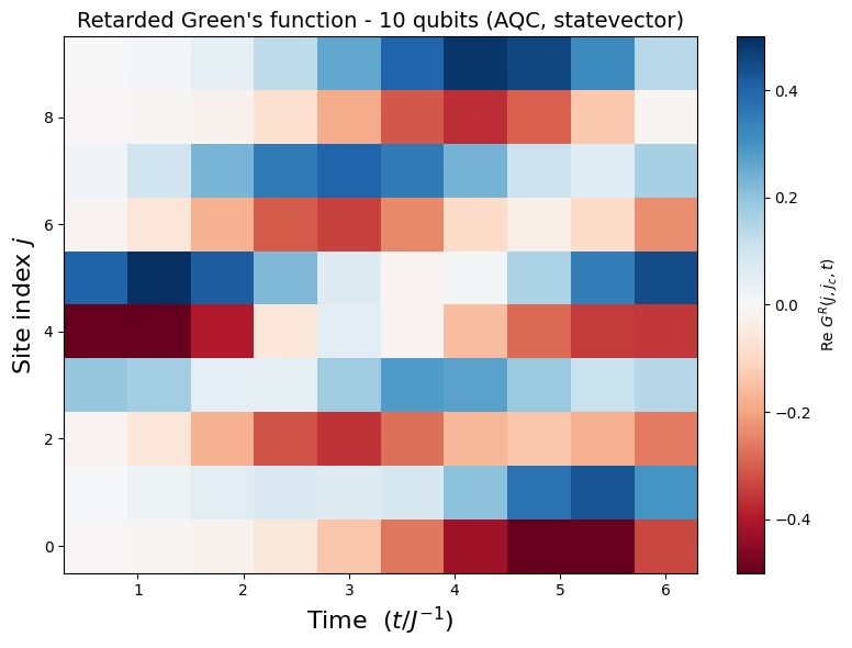
Fourier-transform the Green's function into , mirror-symmetrize, and clip negatives: the standard neutron post-processing. Mirroring is exact because for this model, and the negative values that survive are artifacts of Fourier-transforming a finite, discretely sampled time series, so they are clipped to zero. On this small exact run the two-spinon continuum is only coarsely resolved, but the machinery is identical to the hardware run below.
q_res, w_res = 100, 100
spectrum = get_spectrum(n, Gjjc, dt, time_steps, q_res, w_res)
spectrum = -(spectrum + spectrum[:, ::-1]) / 2  # mirror symmetry
spectrum = np.clip(spectrum, a_min=0, a_max=None)  # clip negatives

plot_green(
    n,
    Gjjc,
    time_steps,
    dt,
    title=f"Retarded Green's function - {n} qubits (AQC, statevector)",
)
plot_spectrum(
    spectrum,
    dt,
    q_res,
    w_res,
    lower_bound=True,
    upper_bound=True,
    title=f"Dynamical structure factor - {n} qubits (AQC, statevector)",
)
Output:
Large-scale hardware example
The same workflow scales up without changing any of the science code: a 30-site chain, twice the Trotter depth (20 steps), a compression plan that varies the ansatz depth (a deeper ansatz for the later, more-entangled steps), and execution on a real IBM Quantum processor with the function's built-in error mitigation (dynamical decoupling, Pauli twirling, and twirled readout error extinction, or TREX). We walk through the same four steps as the simulator example, reusing the fn handle from Setup.
Small scale | Large scale | |
|---|---|---|
| Qubits | 10 | 30 |
| Trotter steps | 10 | 20 |
| AQC segments (1-layer + 2-layer) | 3 + 2 = 5 | 6 + 4 = 10 |
| Ground-state ansatz layers | 3 | 5 |
| MPS max bond dimension | 32 | 128 |
| Backend | statevector | QPU with DD, Pauli twirling, and TREX |
Step 1: Map classical inputs to a quantum problem
Build the same KCuF Heisenberg SparsePauliOp and prepare the ground state, now with a deeper gs_layers=5 ansatz for the longer chain, then bake in the neutron kick at the center site. This is identical to the small-scale mapping, just at .
Expect a lower ground-state fidelity than the 10-site run: around 0.82 here against 0.98 above, because five HVA layers cannot fully capture a 30-site ground state. That is expected rather than a failure, and the original tutorial accepts roughly 0.65 at 50 sites for the same reason. Raising gs_layers or the COBYQA iteration cap improves it, at extra classical cost.
n = 30
dt = 0.6
time_steps = 20
center = n // 2 - 1

# Same MPS settings as the original large-scale run: a larger bond for the
# longer, more-entangled chain (shared by GS prep and AQC compression).
mps_max_bond = 128
mps_cutoff = 1e-8

# Same KCuF3 Hamiltonian and ground-state prep, on a larger chain
H = SparsePauliOp.from_sparse_list(
    [(p, [i, i + 1], 0.25) for i in range(n - 1) for p in ("XX", "YY", "ZZ")],
    num_qubits=n,
)
gs_circuit = prepare_ground_state(
    n, gs_layers=5, max_bond=mps_max_bond, cutoff=mps_cutoff
)
gs_circuit.rz(np.pi / 2, center)  # neutron kick at the center site
print(
    f"Prepared {n}-qubit ground state with the neutron kick at site {center}."
)
Output:
DMRG ground-state energy: -13.111355
GS fidelity: 0.8201
Prepared 30-qubit ground state with the neutron kick at site 14.
Steps 2 and 3: Compress and execute with the function template
The same single call as the simulator example, now with backend_name pointing at a real IBM Quantum processor, so the function transpiles and executes there. The compression plan varies the ansatz depth: the first 6 (low-entanglement) Trotter steps compress into a shallow 1-layer ansatz, the next 4 into a deeper 2-layer ansatz, and the remaining 10 of the 20 steps run as plain Trotter. aqc_options raises the MPS bond dimension to max_bond=128 for the longer, more-entangled chain (matching the original), keeping the same L-BFGS-B optimizer capped at 100 iterations. The estimator_options turn on the built-in error mitigation: dynamical decoupling (XY4), gate twirling, and TREX measurement mitigation. The function's defaults already match the original tutorial for all of these except the TREX learning budget (measure_noise_learning), which is the only genuine difference. The whole block is still written out because a caller-supplied estimator_options replaces the function's defaults wholesale instead of merging into them, so omitting a key would fall back to the Qiskit Runtime default rather than the function's.
# Steps 2 + 3: the function compresses (varied ansatz) and executes on hardware.
job = fn.run(
    t_steps=time_steps,
    aqc_segments=[
        {
            "n_steps": 6,
            "ansatz_steps": 1,
        },  # early steps -> shallow 1-layer ansatz
        {
            "n_steps": 4,
            "ansatz_steps": 2,
        },  # later steps -> deeper 2-layer ansatz
    ],
    aqc_options={
        "max_bond": mps_max_bond,  # 128 for the longer chain
        "cutoff": mps_cutoff,
        "optimizer_settings": {
            "method": "L-BFGS-B",
            "jac": True,
            "options": {"maxiter": 100},
        },
    },
    dt=dt,
    hamiltonian=H,
    initial_state=gs_circuit,
    backend_name="ibm_pittsburgh",
    # Mitigation settings from the original tutorial. Only the two
    # measure_noise_learning values differ from the function's defaults; the rest
    # restates them, because a caller-supplied estimator_options dict replaces the
    # function's defaults wholesale rather than merging into them.
    estimator_options={
        "environment": {"job_tags": ["TUT-SNS"]},
        "dynamical_decoupling": {"enable": True, "sequence_type": "XY4"},
        "twirling": {
            "enable_gates": True,
            "num_randomizations": 1000,
            "shots_per_randomization": 128,
        },
        "resilience": {
            "measure_mitigation": True,
            "measure_noise_learning": {
                "num_randomizations": 32,
                "shots_per_randomization": 100,
            },
        },
    },
)
print("job id (save this to reconnect later):", job.job_id)
Output:
job id (save this to reconnect later): 43ed8d07-6d7d-4f33-b70a-7f31b765b310
The large-scale run is not quick, and most of the time is classical rather than on the QPU. The AQC compression runs inside the function before anything reaches the QPU: at 30 sites with max_bond=128 that took close to four hours in our run, against the roughly 18 minutes of QPU time quoted in the Usage estimate above. Queue wait is on top of both. You do not need to keep this notebook or kernel open while it runs.
Copy the job id printed above and save it. The next three cells let you pick the run back up later:
- Reconnect, only needed in a new kernel session: re-run the Setup cells to recreate
serverless, then rebuild thejobhandle from the id you saved. Skip this cell if you are still in the session where you submitted, because the handle is already live. - Check status: re-run until it reports
DONE. - Fetch the result: run only once the status is
DONE.
The reconnect cell below carries the job id from our own run. Paste yours over there:
# Reconnect to a previously submitted job by its id. Only needed in a NEW kernel
# session; if you are still in the session where you submitted, the `job` handle
# above is already live, so skip this cell. Replace the id below with your own.
job = serverless.get_job_by_id("<your job id>")
# Check where the job is. Re-run this until it reports DONE before fetching the
# result below: OPTIMIZING_FOR_HARDWARE -> WAITING_FOR_QPU -> EXECUTING_QPU ->
# POST_PROCESSING -> DONE.
print(job.status())Output:
DONE
# Run this only once the status cell above reports DONE. result() blocks until
# the job finishes, so calling it earlier just waits (possibly for hours).
result = job.result()
print(
    "AQC fidelities:",
    {k: round(v, 4) for k, v in result["metadata"]["aqc_fidelities"].items()},
)

ev = np.array(result["expectation_values"])
Gjjc = ev[1:]  # drop the t = 0 row -> shape (time_steps, n)
Output:
AQC fidelities: {'1': 1.0, '2': 0.9994, '3': 0.9944, '4': 0.9853, '5': 0.9747, '6': 0.959, '7': 0.9495, '8': 0.9542, '9': 0.9533, '10': 0.9451}
Step 4: Post-process and return result in desired classical format
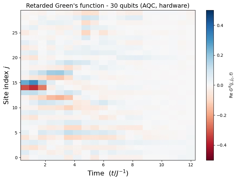
Identical post-processing to the simulator run: Fourier-transform the Green's function into , mirror-symmetrize, and clip negatives. With the longer chain and evolution the two-spinon continuum is far better resolved. It should fill the band between the dashed bounds, brightest near .
n = job.result()["metadata"]["n"]
q_res, w_res = 100, 100
spectrum = get_spectrum(n, Gjjc, dt, time_steps, q_res, w_res)
spectrum = -(spectrum + spectrum[:, ::-1]) / 2  # mirror symmetry
spectrum = np.clip(spectrum, a_min=0, a_max=None)  # clip negatives

plot_green(
    n,
    Gjjc,
    time_steps,
    dt,
    title=f"Retarded Green's function - {n} qubits (AQC, hardware)",
)
plot_spectrum(
    spectrum,
    dt,
    q_res,
    w_res,
    lower_bound=True,
    upper_bound=True,
    title=f"Dynamical structure factor - {n} qubits (AQC, hardware)",
)
Output:
Appendix: How the workflow scales
The hardware example above runs a single chain length. The three spectra below come from earlier hardware runs of this same workflow on ibm_pittsburgh at 10, 20, and 30 sites, with every other input held fixed: 20 Trotter steps at dt = 0.6, the compression plan of 6 one-layer plus 4 two-layer segments, and max_bond = 128. These are recorded results, not output from the cells above.
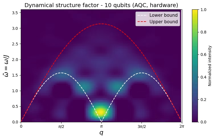
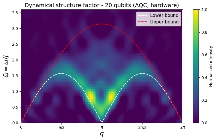
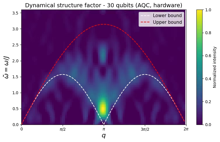
All three recover the two-spinon continuum, brightest at and bounded by the dashed curves, so the physics holds at every size. What changes with chain length is a tradeoff rather than a straight improvement. Momentum resolution sharpens as , so 30 sites map the shape of the continuum far more finely than 10 can. Signal quality moves the other way: longer chains mean deeper circuits, so noise accumulates, contrast fades, and spurious weight leaks outside the bounds.
The two halves of the workflow scale differently in cost as well:
Qubits | Classical (build + AQC) | QPU usage |
|---|---|---|
| 10 | 4m 3s | 14m 21s |
| 20 | 24m 52s | 15m 58s |
| 30 | 230m 57s (about 3h 51m) | 17m 39s |
Queue time is not counted in either column. The classical stage climbs steeply, roughly 6 times from 10 to 20 qubits and another 9 times to 30, dominated by the AQC fidelity optimization at max_bond = 128. QPU usage grows only about 1.2 times across the same range, because the circuit count and shot budget follow t_steps and the twirling settings rather than the qubit count.
Next steps
- Adapt this workflow to your own system: the function is Hamiltonian-agnostic, so a different
SparsePauliOp, initial state, or set of observables runs the same PRE → FUNCTION → POST pipeline. See the full input/output contract in the AQC Dynamics Template. - Read the paper this benchmark comes from: Lee et al., Benchmarking quantum simulation with neutron-scattering experiments (arXiv:2603.15608).
- Compare with the original "Simulate neutron scattering" tutorial, the inline workflow this one ports onto a deployed function template.
- Go deeper on the error mitigation and suppression techniques applied on the hardware run: dynamical decoupling, Pauli twirling, and TREX.