Quantum approximate multi-objective optimization
Usage estimate: about 10 minutes on an IBM Heron processor.
Learning outcomes
This tutorial solves a cardinality-constrained portfolio optimization problem: Given the constraint of holding exactly assets, balance risk, return, and diversification objectives to find the set of optimal portfolios.
After completing this tutorial, you can expect to understand:
- How to express a portfolio-selection problem with three competing objectives — low risk, high return, and good diversification — as a quantum optimization problem.
- How a single QAOA circuit, swept over a set of objective weights, traces out a Pareto front of optimal trade-off portfolios.
- How an XY mixer enforces a "choose exactly K assets" constraint for free, so no penalty term is needed.
- How to train the circuit's angles with a matrix-product-state simulator at a scale too large to optimize exactly, following Kotil et al. (arXiv:2503.22797).
Prerequisites
It is recommended that you are familiar with:
- The Qiskit patterns workflow (map, optimize, execute, post-process).
- The basics of QAOA.
Background
A portfolio manager rarely optimizes a single number. They want returns to be high, risk (the variance of those returns) to be low, and the holdings spread across sectors so the portfolio is not over-exposed to any one part of the market. These goals pull against each other: the highest-return assets are often the most volatile, and concentrating in one hot sector hurts diversification.
There is no single "best" portfolio. Instead there is a Pareto front: the set of portfolios for which you cannot improve one objective without giving up another. Our goal is to map out that front so a decision-maker can pick the trade-off they prefer.
We pose the problem as choosing exactly assets out of (each asset is either in or out — one qubit per asset). Three Hamiltonians encode the three objectives. We combine them with weights that live on a simplex (they sum to one), and a QAOA sampler returns good portfolios for each weight choice. Sweeping the weights sweeps the relative importance of risk vs. return vs. diversification, and the union of all the sampled portfolios traces the Pareto front.
We first walk through the whole workflow on a small 8-asset example we can verify by brute force, then run the identical method on a 40-asset instance sized for quantum hardware.
Requirements
Before starting this tutorial, be sure you have the following installed:
- Qiskit SDK v2.0 or later, with visualization support
- Qiskit Runtime v0.22 or later (
pip install qiskit-ibm-runtime) - Qiskit Aer (
pip install qiskit-aer) - The optimization mapper and training pipeline (
qiskit-addon-opt-mapper,qaoa-training-pipeline) moocorefor Pareto-front and hypervolume calculations (pip install moocore)
Setup
Import the libraries used throughout the tutorial and fix a random seed for reproducibility.
import numpy as np
import matplotlib.pyplot as plt
from math import comb
from moocore import hypervolume, filter_dominated, is_nondominated

from qiskit import QuantumCircuit
from qiskit.circuit import ParameterVector
from qiskit.circuit.library import qaoa_ansatz
from qiskit.quantum_info import SparsePauliOp
from qiskit.transpiler import generate_preset_pass_manager
from qiskit_aer.primitives import SamplerV2 as AerSampler
from qiskit_addon_opt_mapper.problems import OptimizationProblem
from qaoa_training_pipeline.training import ScipyTrainer
from qaoa_training_pipeline.evaluation import (
    StatevectorEvaluator,
    MPSAerEvaluator,
)

np.random.seed(42)
sampler = AerSampler(seed=42)  # local simulator for the small-scale example
print("Setup complete.")
Output:
Setup complete.
Small-scale simulator example
We start with 8 assets drawn from 6 sectors and select exactly of them. With only 8 assets there are just valid portfolios, so we can later check the quantum result against an exhaustive search.
Step 1: Map classical inputs to a quantum problem
Each asset is one qubit; a bitstring like 10110010 is a portfolio (the 1s are the assets we hold). We need three ingredients: the market data, the three objective Hamiltonians, and a circuit that only ever proposes portfolios with exactly assets.
# --- Small-scale universe: 8 assets across 6 sectors ---
tickers = ["AAPL", "XOM", "JPM", "JNJ", "KO", "AMT", "AMZN", "SLB"]
sectors = [
    "Tech",
    "Energy",
    "Finance",
    "Health",
    "Staples",
    "REIT",
    "Tech",
    "Energy",
]
n_assets = len(tickers)
K = 4  # choose exactly K assets
n_obj = 3  # risk, return, diversification

# Annualized expected returns
mu = np.array([0.28, 0.12, 0.22, 0.05, 0.08, 0.10, 0.32, 0.15])

# Annualized covariance matrix (the "risk" model)
sigma = np.array(
    [
        [0.070, 0.010, 0.020, 0.008, 0.005, 0.012, 0.045, 0.011],
        [0.010, 0.065, 0.015, 0.006, 0.004, 0.008, 0.009, 0.050],
        [0.020, 0.015, 0.055, 0.010, 0.007, 0.015, 0.018, 0.014],
        [0.008, 0.006, 0.010, 0.030, 0.012, 0.009, 0.007, 0.005],
        [0.005, 0.004, 0.007, 0.012, 0.025, 0.006, 0.004, 0.003],
        [0.012, 0.008, 0.015, 0.009, 0.006, 0.045, 0.011, 0.007],
        [0.045, 0.009, 0.018, 0.007, 0.004, 0.011, 0.085, 0.010],
        [0.011, 0.050, 0.014, 0.005, 0.003, 0.007, 0.010, 0.072],
    ]
)

# Diversification score: number of cross-sector pairs in the portfolio.
# D[i,j] = 0.5 when assets i and j are in different sectors, so x^T D x counts
# the cross-sector pairs. More cross-sector pairs = better diversified.
D = np.array(
    [
        [1.0 if sectors[i] != sectors[j] else 0.0 for j in range(n_assets)]
        for i in range(n_assets)
    ]
)
np.fill_diagonal(D, 0.0)
D = D / 2

print(f"{n_assets} assets, choose K={K}, {n_obj} objectives")
for t, s, m in zip(tickers, sectors, mu):
    print(f"  {t:5s} ({s:8s})  expected return {m:5.0%}")
Output:
8 assets, choose K=4, 3 objectives
  AAPL  (Tech    )  expected return   28%
  XOM   (Energy  )  expected return   12%
  JPM   (Finance )  expected return   22%
  JNJ   (Health  )  expected return    5%
  KO    (Staples )  expected return    8%
  AMT   (REIT    )  expected return   10%
  AMZN  (Tech    )  expected return   32%
  SLB   (Energy  )  expected return   15%
# Each objective becomes a Hamiltonian whose lowest-energy bitstrings are the
# best portfolios for that objective. The opt-mapper turns a plain
# min/max problem over binary variables into the equivalent Ising operator.
def build_risk_hamiltonian(sigma, n):
    """Minimize portfolio variance x^T sigma x  (quadratic -> ZZ terms)."""
    prob = OptimizationProblem("risk")
    prob.binary_var_list(n)
    prob.minimize(quadratic=sigma)
    op, _ = prob.to_ising()
    return op.simplify()


def build_return_hamiltonian(mu, n):
    """Maximize expected return mu . x  (linear -> Z terms)."""
    prob = OptimizationProblem("return")
    prob.binary_var_list(n)
    prob.maximize(linear=mu)
    op, _ = prob.to_ising()
    return op.simplify()


def build_diversity_hamiltonian(D, n):
    """Maximize cross-sector pairs x^T D x  (quadratic -> ZZ terms)."""
    prob = OptimizationProblem("diversity")
    prob.binary_var_list(n)
    prob.maximize(quadratic=D)
    op, _ = prob.to_ising()
    return op.simplify()


H_risk = build_risk_hamiltonian(sigma, n_assets)
H_return = build_return_hamiltonian(mu, n_assets)
H_diversity = build_diversity_hamiltonian(D, n_assets)
cost_ops = [H_risk, H_return, H_diversity]

for name, op in zip(["risk", "return", "diversity"], cost_ops):
    print(f"H_{name:10s}: {op.size} Pauli terms")
Output:
H_risk      : 36 Pauli terms
H_return    : 8 Pauli terms
H_diversity : 34 Pauli terms
Enforcing "exactly K assets" without a penalty. A common trick is to add a penalty term that punishes portfolios of the wrong size, but that couples every qubit to every other qubit — an all-to-all circuit that does not fit on hardware. Instead we use an XY mixer, which only ever moves the QAOA state between bitstrings of the same Hamming weight. If we start in a state that already has assets selected, every portfolio the circuit explores also has exactly assets. The constraint is built into the circuit's structure, for free.
We prepare the starting state cheaply: rotate each qubit so it is "on" with probability . Restricted to the -asset outcomes, this reproduces the ideal equal-weight (Dicke) state, so we simply keep the measured bitstrings that have exactly ones — a step called post-selection.
def xy_mixer(n):
    """Line XY mixer: couples neighboring qubits with XX+YY. Conserves the number
    of selected assets (Hamming weight), so cardinality is preserved automatically.
    Using a line (not a full ring) keeps the circuit shallow and hardware-friendly."""
    terms = [
        (pauli, [i, i + 1], 1) for i in range(n - 1) for pauli in ("XX", "YY")
    ]
    return SparsePauliOp.from_sparse_list(terms, n)


def product_init(n, k):
    """Cheap initial state: each qubit rotated so P(selected) = k/n. Zero two-qubit
    gates. Post-selecting its weight-k outcomes reproduces the ideal Dicke state."""
    qc = QuantumCircuit(n)
    theta = 2 * np.arcsin(np.sqrt(k / n))
    for q in range(n):
        qc.ry(theta, q)
    return qc


# Combine the three objectives with weights c (bound later, at sampling time).
p_layers = 1
c = ParameterVector("c", n_obj)
combined_cost_op = sum(
    c[k] * H_k for k, H_k in enumerate(cost_ops)
).simplify()

ansatz = qaoa_ansatz(
    combined_cost_op,
    reps=p_layers,
    initial_state=product_init(n_assets, K),
    mixer_operator=xy_mixer(n_assets),
)
ansatz.measure_all()

betas = [p for p in ansatz.parameters if p.name.startswith("β")]
gammas = [p for p in ansatz.parameters if p.name.startswith("γ")]
print(f"Qubits: {ansatz.num_qubits} | QAOA layers: {p_layers}")
print(
    f"Tunable angles: {len(betas)} beta + {len(gammas)} gamma, plus {n_obj} objective weights"
)
Output:
Qubits: 8 | QAOA layers: 1
Tunable angles: 1 beta + 1 gamma, plus 3 objective weights
Step 2: Optimize problem for quantum hardware execution
Before running, the abstract circuit is transpiled into hardware-native gates. At this small scale we just inspect the cost: how deep is the circuit and how many two-qubit gates does it use? (Two-qubit gates are the main source of noise on real devices.)
# Bind dummy angle values so we can transpile and measure the circuit's size.
dummy = {p: 0.1 for p in ansatz.parameters}
test_pm = generate_preset_pass_manager(optimization_level=1)
test_qc = test_pm.run(ansatz.assign_parameters(dummy))

print(f"Circuit depth          : {test_qc.depth()}")
print(
    f"Two-qubit gate depth   : {test_qc.depth(lambda x: len(x.qubits) > 1)}"
)
print(f"Two-qubit gate count   : {test_qc.num_nonlocal_gates()}")
Output:
Circuit depth          : 25
Two-qubit gate depth   : 23
Two-qubit gate count   : 42
Step 3: Execute using Qiskit primitives
Two stages. First we train the QAOA angles once, using equal objective weights, with an exact statevector simulator — this finds good values. Then we sweep many weight vectors across the simplex and sample the circuit at each, collecting candidate portfolios. Because only the objective weights change between sweeps (not the trained angles), all the weight vectors are submitted in a single batched job.
# Train the angles with equal objective weights.
# The trainer maximizes energy, so we negate the (to-be-minimized) objective sum.
training_op = sum(-1.0 / n_obj * H_k for H_k in cost_ops).simplify()

# Linear-ramp initialization (Zhou et al., arXiv:2101.05742)
dt = 0.75
grid = np.arange(1, p_layers + 1) - 0.5
init_params = np.concatenate((1 - grid * dt / p_layers, grid * dt / p_layers))

trainer = ScipyTrainer(
    StatevectorEvaluator(), minimize_args={"options": {"maxiter": 300}}
)
print("Training QAOA angles (exact statevector)...")
result_train = trainer.train(
    cost_op=training_op,
    mixer=xy_mixer(n_assets),
    initial_state=product_init(n_assets, K),
    params0=init_params,
)
opt = result_train["optimized_params"]
opt_betas, opt_gammas = opt[:p_layers], opt[p_layers:]
print(f"Trained beta : {opt_betas}")
print(f"Trained gamma: {opt_gammas}")
Output:
Training QAOA angles (exact statevector)...
Trained beta : [3.329186967386619]
Trained gamma: [3.4449804324291033]
def random_uniform_simplex(n_samples, n_obj=3):
    """n_samples weight vectors spread uniformly over the (n_obj-1)-simplex."""
    s = np.zeros((n_samples, n_obj + 1))
    s[:, 1:-1] = np.random.rand(n_samples, n_obj - 1)
    s[:, -1] = 1
    s = np.sort(s, axis=1)
    return np.diff(s, axis=1)


# Bind the trained angles, leaving the objective weights c free for the sweep.
param_map = {betas[i]: opt_betas[i] for i in range(p_layers)}
param_map.update({gammas[i]: opt_gammas[i] for i in range(p_layers)})
ansatz_bound = ansatz.assign_parameters(param_map)

n_samples, shots = 200, 500
c_vecs = random_uniform_simplex(n_samples, n_obj)

print(f"Sampling {n_samples} weight vectors x {shots} shots...")
result = sampler.run([(ansatz_bound, c_vecs)], shots=shots).result()

# Collect every distinct bitstring seen across all weight vectors.
all_bitstrings = set()
for s in range(n_samples):
    for bs in result[0].data.meas.get_counts(s):
        all_bitstrings.add(bs.replace(" ", ""))
print(f"Distinct portfolios sampled: {len(all_bitstrings)}")
Output:
Sampling 200 weight vectors x 500 shots...
Distinct portfolios sampled: 256
Step 4: Post-process and return result in desired classical format
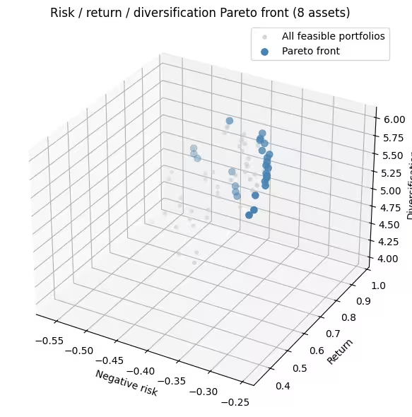
We keep only the feasible portfolios (exactly assets — the post-selection step), score each one on all three objectives, and extract the Pareto front: the portfolios that are not beaten on every objective at once. The hypervolume is a single number summarizing how much objective space the front dominates — bigger is better.
def evaluate_portfolio(bitstring, sigma, mu, D):
    """Score one portfolio on all three objectives (all framed as 'bigger is better')."""
    x = np.array([int(b) for b in bitstring])
    return np.array(
        [
            -(x @ sigma @ x),  # negative risk
            x @ mu,  # return
            x @ D @ x,
        ]
    )  # diversification (cross-sector pairs)


# Post-select feasible portfolios, then score them.
feasible = [bs for bs in all_bitstrings if bs.count("1") == K]
fis = np.array([evaluate_portfolio(bs, sigma, mu, D) for bs in feasible])

pareto_front = filter_dominated(fis, maximise=True)
ref_point = fis.min(axis=0)
qmoo_hv = hypervolume(fis, ref=ref_point, maximise=True)

print(
    f"Feasible portfolios found : {len(feasible)} of {comb(n_assets, K)} possible"
)
print(f"Pareto-front portfolios   : {len(pareto_front)}")
print(f"Hypervolume               : {qmoo_hv:.4f}")
Output:
Feasible portfolios found : 70 of 70 possible
Pareto-front portfolios   : 26
Hypervolume               : 0.2487
fig = plt.figure(figsize=(8, 6))
ax = fig.add_subplot(111, projection="3d")
ax.scatter(
    fis[:, 0],
    fis[:, 1],
    fis[:, 2],
    c="lightgray",
    s=12,
    label="All feasible portfolios",
)
ax.scatter(
    pareto_front[:, 0],
    pareto_front[:, 1],
    pareto_front[:, 2],
    c="steelblue",
    s=45,
    label="Pareto front",
)
ax.set_xlabel("Negative risk")
ax.set_ylabel("Return")
ax.set_zlabel("Diversification")
ax.set_title("Risk / return / diversification Pareto front (8 assets)")
ax.legend()
plt.tight_layout()
plt.show()
Output:
Large-scale hardware example
Now the same workflow on 40 assets (8 sectors × 5), choosing . Forty qubits is too large to optimize the angles exactly ( amplitudes) and too large to verify by brute force, and a dense circuit would be too deep for current hardware. Several things change, and nothing else about the method does:
- Train the angles with a matrix-product-state (MPS) simulator, not exact statevector. Following the reference (Kotil et al.), we fix the objective weights to equal values, optimize a single β, γ on the MPS simulator, and reuse them for every weighting vector in the sweep. (We train at the size we run — no small-to-large angle transfer.)
- Sparsify the risk model to fit hardware. A full covariance couples all 780 asset pairs. We keep only the strongest, cheapest-to-route couplings using importance-aware QAP truncation, and couple each sector in a light ring for the diversity term — together this keeps the objectives meaningful while holding the circuit to a hardware-friendly size.
- Keep the circuit shallow and score honestly. Routing is stochastic, so we transpile with several seeds and keep the shallowest (free — no quantum time spent). Portfolios are always scored against the true, full objectives — the sparsification only shapes the circuit, not how portfolios are judged.
Why QAP truncation? Keeping each asset's largest couplings by magnitude alone can leave a circuit that is sparse but still awkward to route. QAP truncation instead keeps couplings that are both large and physically close on the chip, so the same gate budget buys a shallower, more hardware-friendly circuit.
Step 1: Map inputs (sparsified for hardware)
import csv
import urllib.request

# Download the committed market-data snapshot from the repo.
# --- 40-asset universe: 8 GICS sectors x 5 tickers (real market data) ---
# Load the committed market-data snapshot (real annualized returns and covariance).
# Values are stored at the precision used to train the shipped QAOA angles
# (mu: 3 dp, sigma: 4 dp), so the pre-trained parameters in instances/ stay exactly valid.

url = "https://raw.githubusercontent.com/Qiskit/documentation/main/datasets/tutorials/qmoo/market_data.csv"
urllib.request.urlretrieve(url, "market_data.csv")

with open("market_data.csv", newline="") as _f:
    _rows = list(csv.reader(_f))

_tickers_csv = _rows[0][2:]  # covariance column order
tickers_40 = [r[0] for r in _rows[1:]]  # asset tickers
mu_40 = np.array(
    [float(r[1]) for r in _rows[1:]]
)  # annualized expected returns
sigma_40 = np.array(
    [[float(v) for v in r[2:]] for r in _rows[1:]]
)  # covariance (risk model)

sectors_40 = [
    "Tech",
    "Tech",
    "Tech",
    "Tech",
    "Tech",
    "Energy",
    "Energy",
    "Energy",
    "Energy",
    "Energy",
    "Finance",
    "Finance",
    "Finance",
    "Finance",
    "Finance",
    "Health",
    "Health",
    "Health",
    "Health",
    "Health",
    "Staples",
    "Staples",
    "Staples",
    "Staples",
    "Staples",
    "Industrials",
    "Industrials",
    "Industrials",
    "Industrials",
    "Industrials",
    "Utilities",
    "Utilities",
    "Utilities",
    "Utilities",
    "Utilities",
    "REIT",
    "REIT",
    "REIT",
    "REIT",
    "REIT",
]
n_assets_40 = len(tickers_40)
K_40 = 6  # choose exactly K assets

sector_names_40 = list(dict.fromkeys(sectors_40))
sect_idx_40 = np.array([sector_names_40.index(s) for s in sectors_40])
# True cross-sector diversification matrix (used for scoring)
D_40 = np.array(
    [
        [
            0.5 if sectors_40[i] != sectors_40[j] else 0.0
            for j in range(n_assets_40)
        ]
        for i in range(n_assets_40)
    ]
)
np.fill_diagonal(D_40, 0.0)
print(
    f"{n_assets_40} assets, {len(sector_names_40)} sectors, choose K={K_40}"
)
# Sparsify the covariance so the risk circuit fits on hardware. A small diagonal
# shift (added after truncation) keeps the risk model positive semidefinite; at fixed
# K it adds the same constant to every portfolio, so it never changes the ranking.
# Importance-aware QAP truncation (Kotil et al. style): place the qubits on a line
# and use a Quadratic Assignment Problem to choose the layout that keeps the
# strongest covariance couplings within routing distance k of the swap network,
# then drop the rest. Unlike a fixed top-k cap, it keeps couplings that are both
# large AND cheap to route.
from scipy.optimize import quadratic_assignment as qap
from qiskit.transpiler.passes.routing.commuting_2q_gate_routing import (
SwapStrategy,
)
k_truncate = (
2 # truncation level: larger k keeps more couplings (deeper circuit)
)
_dist = np.array(
SwapStrategy.from_line(list(range(n_assets_40))).distance_matrix
)
def qap_truncate(Q, k):
w = np.abs(Q.copy())
np.fill_diagonal(w, 0.0)
mask = (_dist <= k).astype(float)
# Seed the QAP solver explicitly (by default it draws from NumPy's global
# RNG, which SciPy is deprecating) so the truncation is reproducible.
perm = qap(-w, mask, options={"rng": np.random.default_rng(42)}).col_ind
keep = mask[np.ix_(perm, perm)]
Qt = Q * keep
np.fill_diagonal(Qt, np.diag(Q))
return Qt
sigma_sparse = qap_truncate(sigma_40, k_truncate)
print(
f"QAP truncation (k={k_truncate}): risk edges kept = "
f"{(np.count_nonzero(sigma_sparse) - n_assets_40) // 2}"
)
ridge = max(0.0, -np.linalg.eigvalsh(sigma_sparse)[0]) + 1e-6
sigma_sparse = sigma_sparse + ridge * np.eye(n_assets_40)
# Diversity: couple each sector's assets in a ring (sparse stand-in for the
# same-sector pair count). Scoring still uses the true cross-sector matrix D_40.
def build_same_sector_hamiltonian(D_same, n):
prob = OptimizationProblem("diversity_sparse")
prob.binary_var_list(n)
prob.minimize(quadratic=D_same)
op, _ = prob.to_ising()
return op.simplify()
D_ring = np.zeros((n_assets_40, n_assets_40))
for s in set(sect_idx_40):
members = np.where(sect_idx_40 == s)[0]
for k in range(len(members)):
i, j = members[k], members[(k + 1) % len(members)]
D_ring[i, j] = D_ring[j, i] = 0.5
H_risk_40 = build_risk_hamiltonian(sigma_sparse, n_assets_40)
H_return_40 = build_return_hamiltonian(mu_40, n_assets_40)
H_diversity_40 = build_same_sector_hamiltonian(D_ring, n_assets_40)
cost_ops_40 = [H_risk_40, H_return_40, H_diversity_40]
n_zz = sum(
1 for p in sum(cost_ops_40).simplify().paulis if str(p).count("Z") == 2
)
print(
f"Cost-layer interactions: {n_zz} (dense would be {n_assets_40*(n_assets_40-1)//2})"
)Output:
QAP truncation (k=2): risk edges kept = 78
Cost-layer interactions: 102 (dense would be 780)
Steps 2-3: train the angles, then build and submit the hardware job
Forty qubits is too large to optimize the angles exactly, so we train one β, γ on a matrix-product-state simulator at equal objective weights and reuse them across the sweep (the loaded values below). The cost-layer angle is small here: the circuit applies a gentle bias rather than a sharp projection.
import json
from qiskit_ibm_runtime import QiskitRuntimeService, SamplerV2

# Pre-trained angles loaded from a file (training is slow; QDC pattern).
# Set load_params_file = False to retrain in-notebook.
load_params_file = True
params_url = "https://raw.githubusercontent.com/Qiskit/documentation/main/datasets/tutorials/qmoo/qaoa_params.json"
params_path = "qaoa_params.json"
if load_params_file:
    urllib.request.urlretrieve(params_url, params_path)
    qaoa_params = json.load(open(params_path))
    p_layers_hw = qaoa_params["p_layers"]
    opt_betas_40, opt_gammas_40 = qaoa_params["betas"], qaoa_params["gammas"]
else:
    # Same workflow as the small-scale example: qaoa_training_pipeline's MPSAerEvaluator
    # evaluates the QAOA energy on Aer's MPS simulator and supports the XY mixer.
    # As in the small-scale example the trainer maximizes energy, so we negate the
    # (to-be-minimized) objective sum; the 1/n_obj scaling matches the equal-weight
    # point of the sweep, so the trained gamma transfers directly to the weighted circuits.
    p_layers_hw = 1
    training_op_40 = sum(-1.0 / n_obj * H_k for H_k in cost_ops_40).simplify()

    dt = 0.75
    grid = np.arange(1, p_layers_hw + 1) - 0.5
    init_params_40 = np.concatenate(
        (1 - grid * dt / p_layers_hw, grid * dt / p_layers_hw)
    )

    trainer_40 = ScipyTrainer(
        MPSAerEvaluator({"matrix_product_state_max_bond_dimension": 24}),
        minimize_args={"options": {"maxiter": 80}},
    )
    print("Training QAOA angles (MPS simulator)...")
    result_train_40 = trainer_40.train(
        cost_op=training_op_40,
        mixer=xy_mixer(n_assets_40),
        initial_state=product_init(n_assets_40, K_40),
        params0=init_params_40,
    )
    opt_40 = result_train_40["optimized_params"]
    opt_betas_40, opt_gammas_40 = (
        list(opt_40[:p_layers_hw]),
        list(opt_40[p_layers_hw:]),
    )
    import os

    os.makedirs(os.path.dirname(params_path), exist_ok=True)
    json.dump(
        {
            "p_layers": p_layers_hw,
            "betas": opt_betas_40,
            "gammas": opt_gammas_40,
        },
        open(params_path, "w"),
        indent=2,
    )
    print(
        f"Trained angles saved to {params_path} (set load_params_file=True to reuse)."
    )

c40 = ParameterVector("c", n_obj)
combined_cost_op_40 = sum(
    c40[k] * H_k for k, H_k in enumerate(cost_ops_40)
).simplify()
qc_40 = qaoa_ansatz(
    combined_cost_op_40,
    reps=p_layers_hw,
    initial_state=product_init(n_assets_40, K_40),
    mixer_operator=xy_mixer(n_assets_40),
)
qc_40.measure_all()
b40 = [p for p in qc_40.parameters if p.name.startswith("β")]
g40 = [p for p in qc_40.parameters if p.name.startswith("γ")]
pmap = {b40[i]: opt_betas_40[i] for i in range(p_layers_hw)}
pmap.update({g40[i]: opt_gammas_40[i] for i in range(p_layers_hw)})
ansatz_qc_40 = qc_40.assign_parameters(pmap)

service = QiskitRuntimeService()

# only use Heron devices
backend = service.least_busy(min_num_qubits=156)


# SABRE routing is stochastic: different seeds give different depths. Transpilation
# is classical (it costs no QPU time), so we transpile many seeds and keep only the
# shallowest circuit -- a free reduction in two-qubit depth before anything is sent
# to hardware. Only this single best circuit is ever executed.
n_seeds = 24
best = None
depths = []
for seed in range(n_seeds):
    pm = generate_preset_pass_manager(
        optimization_level=3, backend=backend, seed_transpiler=seed
    )
    qc = pm.run(ansatz_qc_40)
    d2 = qc.depth(lambda x: len(x.qubits) > 1)
    depths.append(d2)
    if best is None or d2 < best[0]:
        best = (d2, seed, qc)
isa_qc = best[2]
sd = sorted(depths)
print(
    f"Backend: {backend.name} | {n_seeds} seeds | two-qubit depth "
    f"best/median/worst = {sd[0]}/{sd[len(sd)//2]}/{sd[-1]} (best seed {best[1]})"
)
print(
    f"Selected circuit -> two-qubit gates: {isa_qc.num_nonlocal_gates()}, "
    f"two-qubit depth: {isa_qc.depth(lambda x: len(x.qubits) > 1)}"
)
Output:
Backend: ibm_marrakesh | 24 seeds | two-qubit depth best/median/worst = 220/261/300 (best seed 22)
Selected circuit -> two-qubit gates: 787, two-qubit depth: 220
# Submit one batched job (job mode; a single batch needs no Session).
n_samples_40, shots_40 = (
    24,
    1500,
)  # extra shots: noise lowers the post-selection yield
c_vecs_40 = random_uniform_simplex(n_samples_40, n_obj)
sampler_hw = SamplerV2(mode=backend)
sampler_hw.options.max_execution_time = (
    600  # seconds; guard against runaway jobs
)

# The QAOA angles are already bound; only the objective weights c remain free.
# Assign each weight vector to get one concrete circuit per point on the simplex.
bound_circuits_40 = [
    isa_qc.assign_parameters({c40[k]: cv[k] for k in range(n_obj)})
    for cv in c_vecs_40
]
job_hw = sampler_hw.run([(qc,) for qc in bound_circuits_40], shots=shots_40)
print(
    f"Submitted to {backend.name}: job id {job_hw.job_id()} ({len(bound_circuits_40)} circuits)"
)
Output:
Submitted to ibm_marrakesh: job id d9choesjeosc73fg9ma0 (24 circuits)
Step 4: Post-process into the Pareto front and read off the optimal portfolios
result_hw = job_hw.result()

# Post-select feasible portfolios (exactly K assets), score on the TRUE objectives.
feasible_40 = set()
for s in range(n_samples_40):
    for bs in result_hw[s].data.meas.get_counts():
        bs = bs.replace(" ", "")
        if bs.count("1") == K_40:
            feasible_40.add(bs)


def evaluate_40(bs):
    x = np.array([int(b) for b in bs])
    return np.array([-(x @ sigma_40 @ x), x @ mu_40, x @ D_40 @ x])


fis_40 = np.array([evaluate_40(bs) for bs in feasible_40])
pareto_40 = filter_dominated(fis_40, maximise=True)

# Honesty check: compare against the same number of uniformly-random K-asset portfolios.
rng = np.random.default_rng(0)
rand = set()
while len(rand) < len(feasible_40):
    pick = rng.choice(n_assets_40, K_40, replace=False)
    rand.add("".join("1" if i in pick else "0" for i in range(n_assets_40)))
fis_rand = np.array([evaluate_40(bs) for bs in rand])
ref = np.minimum(fis_40.min(axis=0), fis_rand.min(axis=0))
print(f"Feasible portfolios collected : {len(feasible_40)}")
print(f"Pareto-front portfolios       : {len(pareto_40)}")
print(
    f"Hypervolume  QAOA vs random   : "
    f"{hypervolume(fis_40, ref=ref, maximise=True):.3f}  vs  "
    f"{hypervolume(fis_rand, ref=ref, maximise=True):.3f}"
)
Output:
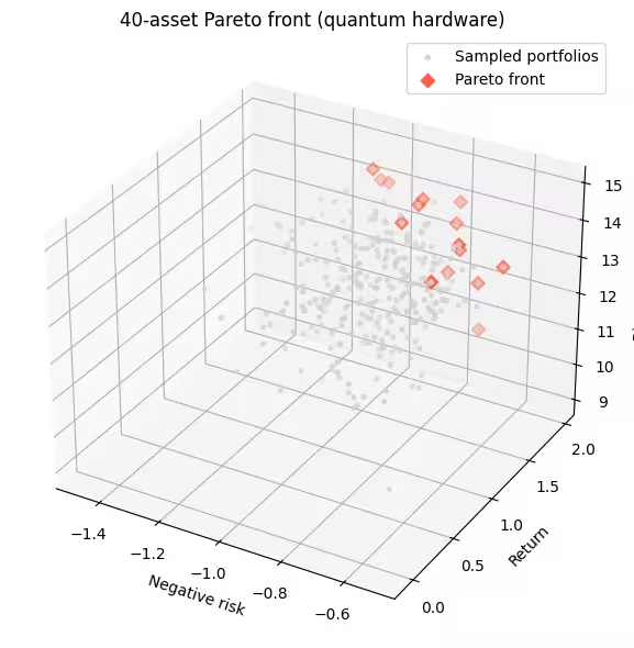
Feasible portfolios collected : 296
Pareto-front portfolios       : 15
Hypervolume  QAOA vs random   : 14.145  vs  12.973
# The answer: the Pareto-optimal portfolios. Every point on the front is optimal in
# the sense that improving one objective requires giving up another -- the front IS the
# set of answers, and a decision-maker picks the trade-off they prefer.
bs_list = list(feasible_40)
# Boolean mask over fis_40; keep_weakly=True also keeps portfolios whose
# objective values tie with a front point (what the strict filter would drop).
mask = is_nondominated(fis_40, maximise=True, keep_weakly=True)
front_bs = [b for b, m in zip(bs_list, mask) if m]
front_f = fis_40[mask]
order = np.argsort(-front_f[:, 1])  # show a span sorted by return
print(f"{mask.sum()} Pareto-optimal portfolios. A representative span:\n")
print(
    f"{'tickers held':40s} {'risk':>7s} {'return':>7s} {'cross-sector':>12s}"
)
for idx in order[:: max(1, len(order) // 12)]:
    held = [tickers_40[i] for i, b in enumerate(front_bs[idx]) if b == "1"]
    print(
        f"{', '.join(held):40s} {-front_f[idx,0]:7.3f} {front_f[idx,1]:7.2f} {int(front_f[idx,2]):12d}"
    )

fig = plt.figure(figsize=(8, 6))
ax = fig.add_subplot(111, projection="3d")
ax.scatter(
    fis_40[:, 0],
    fis_40[:, 1],
    fis_40[:, 2],
    c="lightgray",
    s=8,
    label="Sampled portfolios",
)
ax.scatter(
    pareto_40[:, 0],
    pareto_40[:, 1],
    pareto_40[:, 2],
    c="tomato",
    marker="D",
    s=40,
    label="Pareto front",
)
ax.set_xlabel("Negative risk")
ax.set_ylabel("Return")
ax.set_zlabel("Diversification")
ax.set_title("40-asset Pareto front (quantum hardware)")
ax.legend()
plt.tight_layout()
plt.show()
Output:
15 Pareto-optimal portfolios. A representative span:

tickers held                                risk  return cross-sector
NVDA, CVX, WMT, CAT, HON, NEE              1.065    1.97           14
NVDA, BLK, WMT, GE, NEE, AEP               1.038    1.97           14
MS, JNJ, WMT, CAT, HON, AEP                0.798    1.96           14
JNJ, KO, WMT, CAT, HON, RTX                0.692    1.81           11
XOM, GS, JNJ, KO, GE, RTX                  0.746    1.70           14
NVDA, COP, BLK, PFE, WMT, RTX              1.007    1.64           15
JNJ, KO, WMT, HON, GE, SPG                 0.733    1.54           13
NVDA, KO, HON, RTX, SO, AEP                0.628    1.51           13
AAPL, MS, WMT, HON, AEP, CCI               0.794    1.45           15
JPM, KO, WMT, HON, AEP, SPG                0.664    1.41           14
GS, JNJ, PG, CAT, NEE, CCI                 0.787    1.37           15
MSFT, JNJ, KO, CAT, D, AEP                 0.512    1.35           14
AAPL, EOG, UNH, CAT, AEP, AMT              0.777    1.12           15
XOM, MS, PFE, PG, RTX, DUK                 0.579    1.05           15
MSFT, JNJ, PG, HON, AEP, CCI               0.545    0.57           15
Next steps
If you found this tutorial interesting, you might explore:
- Replace the embedded market data with your own returns and covariance estimates from real price history.
- Increase the number of QAOA layers, or train at 12–16 assets and transfer those angles, to push the hardware front closer to optimal.
- Read Kotil et al., Quantum Approximate Multi-Objective Optimization (Nature Computational Science, 2025), the max-cut study this tutorial adapts to portfolios.
- See the companion unconstrained notebook, which follows Kotil et al. with standard QAOA and the MPS training pipeline.