Refresh backend properties with real-time benchmarking

Usage estimate: 3 minutes on ibm_kingston (NOTE: This is an estimate only. Your runtime might vary.)

Learning outcomes

After completing this tutorial, you can expect to understand the following:

• Why the properties reported by a QPU can lag behind the device's current behavior, and when it is worth re-measuring them yourself
• What each of the five standard characterization experiments (readout, single-qubit randomized benchmarking, layered two-qubit randomized benchmarking, $T_1$, and $T_2$) measures
• How to run the full characterization suite in a single call or step by step, and get back a backend object with refreshed properties
• How to compare the measured properties against the reported ones, and why some differences reflect measurement methodology rather than device drift

Prerequisites

It is recommended that you familiarize yourself with these topics:

• The Qiskit patterns workflow
• Qiskit Runtime execution modes, in particular batch mode
• How to explore QPU information such as backend properties and calibration data

Background

Every IBM Quantum® QPU reports a set of properties that describe how well each of its qubits is currently working: relaxation times ($T_1$), coherence times ($T_2$), readout errors, and one- and two-qubit gate errors. These numbers matter in practice. The transpiler uses them to decide which physical qubits your circuit should run on, error mitigation techniques rely on them, and you might use them to judge whether a device is in good enough shape for an experiment.

The reported properties come from calibration procedures that typically run about once a day. Superconducting qubits, however, can drift on shorter timescales, and transient defects (so-called two-level systems) can temporarily degrade a qubit that looked excellent at calibration time. In addition, a job is often transpiled well before it actually executes, so decisions based on the reported properties can rest on stale information. The tutorial Real-time benchmarking for qubit selection shows how much these properties can fluctuate from day to day, and builds a full characterization workflow by hand from individual Qiskit Experiments.

This tutorial shows the streamlined version of that workflow: the BackendCharacterization utility from Qiskit Device Benchmarking packages the experiment construction, job submission, and curve fitting into a few calls. You spend roughly 70 seconds of QPU time and get back a backend object whose properties reflect the device right now, ready to be compared against the reported values or passed on to downstream tools.

The characterization experiments

The suite measures five properties, each with a standard experiment:

• Readout error (readout): Each qubit is prepared in $|0\rangle$ or $|1\rangle$ and immediately measured. The probability of reading out the wrong state gives the state preparation and measurement (SPAM) error.
• Single-qubit gate error (rb_1q): Randomized benchmarking (RB) runs sequences of random single-qubit Clifford gates that ideally compose to the identity. The way the survival probability decays with sequence length yields the average error per gate, independent of SPAM errors.
• Two-qubit gate error (rb_2q): The same RB idea applied to full layers of non-overlapping two-qubit gates executed simultaneously, as in a layer fidelity experiment. Because many gates run at once, the resulting error rates include crosstalk effects and are closer to what a deep circuit actually experiences.
• $T_1$ (t1): Each qubit is excited and measured after increasing delays. The decay of the excited-state population gives the relaxation time.
• $T_2$ (t2): A Hahn echo experiment puts each qubit in a superposition, applies an echo pulse halfway through a delay, and measures how quickly phase coherence is lost. By default a single echo is used; a multi-echo (CPMG-style) variant is demonstrated at the end of this tutorial.

What refreshing does and does not do

Keep three points in mind when using this workflow:

• The refreshed properties live only in the backend object returned to you. Nothing changes on the device itself or in the calibration data that IBM Quantum reports to other users.
• The measured values are a snapshot taken with a particular methodology. Some of them, notably the layered two-qubit errors and the parallel single-echo $T_2$ values, are measured differently from the reported calibration data, so part of any gap you observe is methodological rather than drift. This tutorial points out where that happens.
• The characterization itself costs QPU time (about 70 seconds for the full suite on a Heron r2 processor), which is the price of up-to-date information.

The workflow follows the four steps of a Qiskit pattern:

• Step 1: Map classical inputs to a quantum problem. Choose the device and the set of properties to measure.
• Step 2: Optimize problem for quantum hardware execution. The utility builds the experiment circuits directly in the device's native gates and parallelizes them across the chip.
• Step 3: Execute using Qiskit primitives. The experiments run as Sampler jobs inside a batch.
• Step 4: Post-process and return result in desired classical format. Fit the measurement data into per-qubit error maps, refresh the backend, and compare the measured properties against the reported ones.

Requirements

Before starting this tutorial, be sure you have the following installed:

• Qiskit SDK v2.0 or later, with visualization support
• Qiskit Runtime v0.40 or later (pip install qiskit-ibm-runtime)
• Qiskit Device Benchmarking, which also installs Qiskit Experiments (pip install git+https://github.com/qiskit-community/qiskit-device-benchmarking.git)

Setup

Import the required libraries.

import logging
import sys

import numpy as np
from qiskit_ibm_runtime import Batch, QiskitRuntimeService

from qiskit_device_benchmarking.utilities.characterization_utils import (
    BackendCharacterization,
    plot_characterization_comparison,
)

The characterization suite builds several experiments, submits multiple jobs, and fits the results, which can take a couple of minutes in total. Enable INFO-level logging so that each stage prints its progress as it happens.

logger = logging.getLogger("qiskit_device_benchmarking")
logger.setLevel(logging.INFO)
logger.addHandler(logging.StreamHandler(stream=sys.stdout))

Small-scale simulator example

This tutorial does not include a simulator example. The workflow measures the physical imperfections of a specific device: how quickly its qubits relax and dephase, and how often its gates and readout fail. An ideal simulator has none of these imperfections, so there is nothing to characterize. You could attach a synthetic noise model to a fake backend, but the experiments would then only recover the numbers you put in yourself. For that reason, we proceed directly to hardware, broken into the four steps of a Qiskit pattern.

Large-scale hardware example

Step 1: Map classical inputs to a quantum problem

In this workflow the "problem" is the device itself: the classical inputs are the QPU you want to characterize and the list of properties to measure, and the quantum experiments are the characterization circuits generated from them.

First, select a backend. This tutorial uses ibm_kingston, a 156-qubit Heron r2 processor; you can substitute any IBM Quantum device you have access to (or pick one with service.least_busy()).

service = QiskitRuntimeService()
device = "ibm_kingston"
backend = service.backend(device)

Next, choose which properties to measure. You can pass any subset of the following experiments:

• readout: SPAM (state preparation and measurement) experiment
• rb_1q: isolated single-qubit randomized benchmarking
• rb_2q: simultaneous two-qubit randomized benchmarking from a layer fidelity experiment
• t2: $T_2$ Hahn echo experiment (a single echo by default)
• t1: $T_1$ relaxation experiment

Running the full suite gives a complete picture of the device; drop entries from the list if you only care about some properties and want to save QPU time.

experiments = ["readout", "rb_1q", "rb_2q", "t1", "t2"]

Step 2: Optimize problem for quantum hardware execution

In most tutorials this is where you would transpile your circuits. Here, BackendCharacterization takes care of that internally: it builds the experiment circuits directly in the device's native gates, runs the single-qubit experiments on all qubits in parallel, and schedules the two-qubit benchmarking over disjoint layers of the coupling map so that the entire device is covered with a handful of jobs. This parallelization is what keeps the whole suite down to about 70 seconds of QPU time.

Initialize the class that manages the workflow:

# Initialize the class used to run the experiments
characterizer = BackendCharacterization(backend)

Step 3: Execute using Qiskit primitives

The run_experiments method builds the circuits and submits them as Sampler jobs. Run it inside a Batch context so that the jobs are scheduled together on the QPU, and the method returns once all jobs have been submitted. (You can also run it outside a batch, or inside a Session.)

# Run the characterization experiments inside a Batch
with Batch(backend=backend):
    jobs = characterizer.run_experiments(experiments=experiments)

Output:

base_primitive.get_mode_service_backend:WARNING:2026-07-14 14:23:02,051: A backend was passed in as the mode but a session context manager is open so this job will run inside this session/batch instead of in job mode.

Building readout experiments
Building 1Q RB experiments
Building 2Q RB experiments
Building T1 experiments
Building T2 experiments
Layered two-qubit RB submitted: ['d9b7tfu6hjac73ffba2g', 'd9b7tjug26ic73dfju3g', 'd9b7u3u6hjac73ffban0', 'd9b7u7rv6alc73csmicg']
Readout job submitted: d9b7u8bv6alc73csmidg
T1 experiment submitted: ['d9b7u8ug26ic73dfjuqg']
T2 (Hahn) experiment submitted: ['d9b7u9fu62qs738othg0']
Single-qubit RB submitted: ['d9b7v8m6hjac73ffbc40', 'd9b7veeg26ic73dfk040']

The method returns the submitted jobs as a dictionary keyed by experiment, which is useful for tracking them on the IBM Quantum Platform dashboard or for debugging.

# Print all the job IDs for debugging purposes
jobs

Output:

{'rb_2q': [<RuntimeJobV2('d9b7tfu6hjac73ffba2g', 'sampler')>,
  <RuntimeJobV2('d9b7tjug26ic73dfju3g', 'sampler')>,
  <RuntimeJobV2('d9b7u3u6hjac73ffban0', 'sampler')>,
  <RuntimeJobV2('d9b7u7rv6alc73csmicg', 'sampler')>],
 'readout': [<RuntimeJobV2('d9b7u8bv6alc73csmidg', 'sampler')>],
 't1': [<RuntimeJobV2('d9b7u8ug26ic73dfjuqg', 'sampler')>],
 't2': [<RuntimeJobV2('d9b7u9fu62qs738othg0', 'sampler')>],
 'rb_1q': [<RuntimeJobV2('d9b7v8m6hjac73ffbc40', 'sampler')>,
  <RuntimeJobV2('d9b7veeg26ic73dfk040', 'sampler')>]}

Step 4: Post-process and return result in desired classical format

Analyze the results

The analyze_results method waits for the jobs to finish and fits the measurement data: exponential decays for $T_1$ and $T_2$, survival-probability decays for the RB experiments, and assignment matrices for readout. It returns a dictionary of error maps, one entry per measured property, each mapping a qubit (or qubit pair) to its measured value.

error_maps = characterizer.analyze_results()

print(f"The following error maps are available: {list(error_maps.keys())}")
readout_q0 = error_maps["readout_error"][0]
print(f"For example, readout error for qubit 0 is {readout_q0}")

Output:

The following error maps are available: ['readout_error', 'oneq_error_x', 'oneq_error_sx', 'lf_error_map', 't1_map', 't2_map']
For example, readout error for qubit 0 is 0.007600000000000051

The maps cover readout error, the single-qubit x and sx gate errors, the layered two-qubit errors (lf_error_map, from the layer fidelity experiment), and the $T_1$ and $T_2$ times in seconds.

Update the backend properties

The update_backend method writes the measured values into the properties of a copy of the backend and returns it. The original backend object keeps the reported calibration data, which lets us compare the two below. Remember that this update is purely local to your Python session; it does not change anything on the device or for other users.

backend_updated = characterizer.update_backend()

Output:

Updating readout error
Updating single-qubit X error
Updating single-qubit SX error
Updating two-qubit error
Updating T1
Updating T2

Compare the measured properties against the reported ones

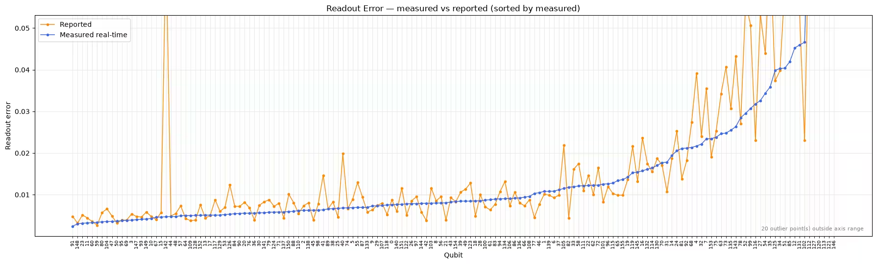
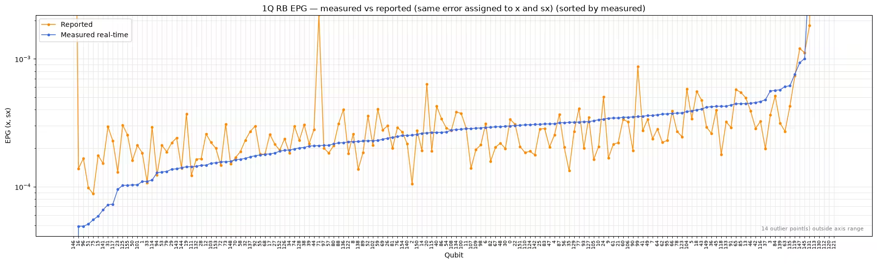
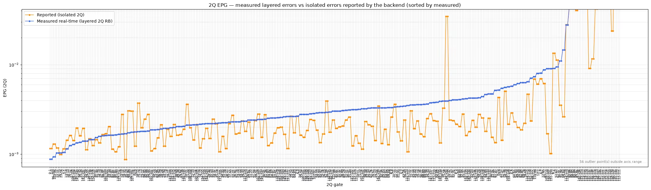
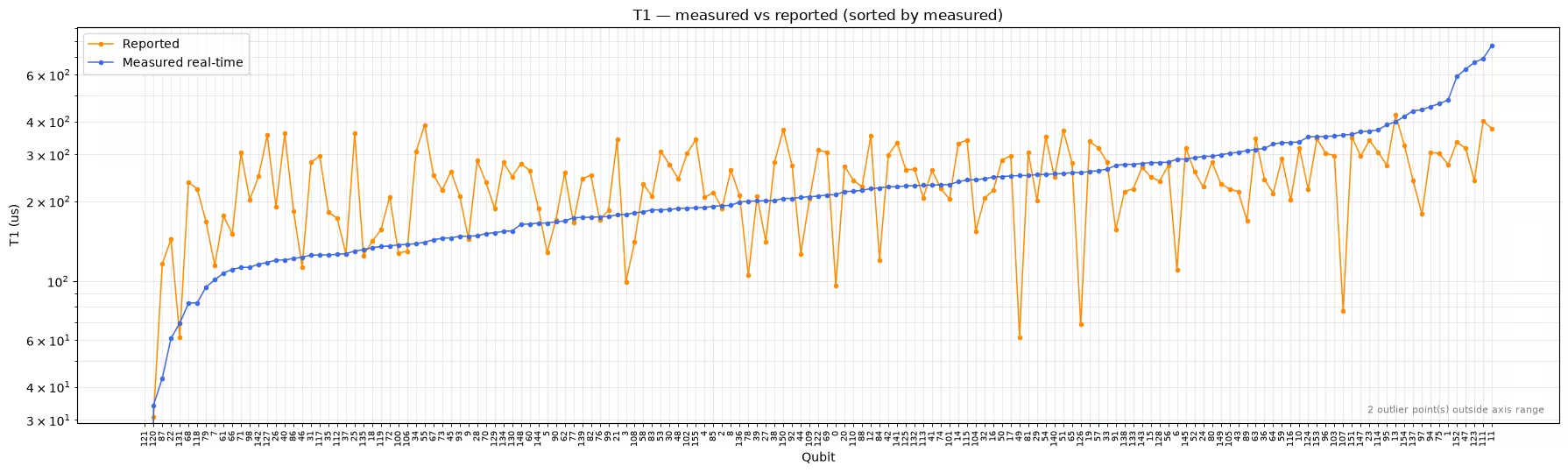
Finally, plot the measured real-time properties against the values the backend reports. In each panel the qubits (or qubit pairs) are sorted by the measured value, so the measured curve is smooth by construction and the scatter of the reported values around it shows where the two disagree. A single plot is shown for single-qubit RB because the same measured error per gate is assigned to both the x and sx gates. Axis limits are chosen from the bulk of the data so that a few extreme outliers do not compress the plots; any points outside the range are counted in an annotation on the plot (or pass ylim to override the limits).

plot_characterization_comparison(
    old_props=backend.properties().to_dict(),
    new_props=backend_updated.properties().to_dict(),
    plots=["readout", "rb_1q", "rb_2q", "t1", "t2"],
)

Output:

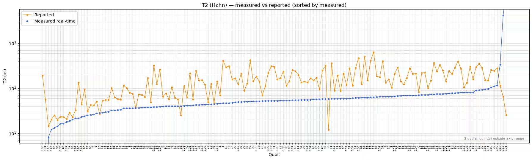
These plots reward a careful reading, because not every gap between the two curves means the device has drifted:

• Readout and single-qubit errors: The measured values track the reported ones for most qubits, with a handful of qubits where the reported value is far off the measured curve. Those localized disagreements are the drift this workflow is designed to catch.
• $T_1$: The two data sets scatter around each other with no systematic offset, which is consistent with $T_1$ fluctuating naturally over time.
• Two-qubit errors: The measured values sit systematically above the reported ones. This is expected rather than alarming: the reported values are measured on isolated gates, while the layer fidelity experiment runs many gates simultaneously and therefore includes crosstalk. The layered numbers are arguably the more relevant ones for deep circuits, but they are not directly comparable to the reported calibration data.
• $T_2$: The measured values sit well below the reported ones for most qubits. Again, methodology plays a large role, as examined in the next section.

Inspect individual experiment results

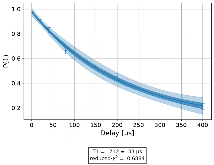
You can also inspect the raw results of the individual characterization experiments through the experiment_data property, which returns the underlying Qiskit Experiments ExperimentData objects. For example, the following displays the measured $T_1$ decay curve of a single qubit, which is useful for checking the quality of a fit before trusting the number it produced.

t1_data = characterizer.experiment_data["t1"]

# Each qubit has its own fit figure
n_figs = len(t1_data.figure_names)
print(f"{n_figs} figures available, e.g. {t1_data.figure_names[0]}")

# Show the T1 decay curve of the first qubit
t1_data.figure(0)

Output:

156 figures available, e.g. T1_Q0_c78ef792.svg

Measure T2 with a dynamical decoupling train

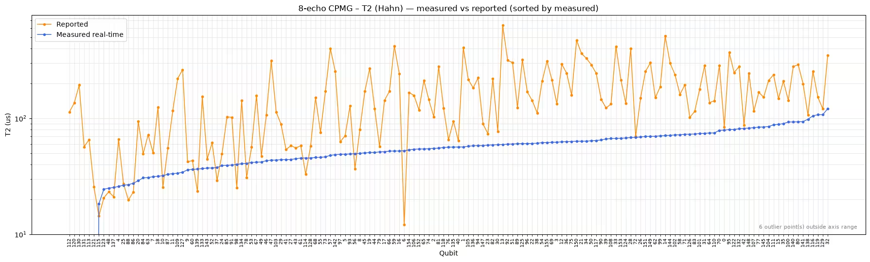
By default the $T_2$ experiment applies a single Hahn echo and measures all qubits in parallel, which, as the comparison plot above showed, can yield noticeably lower $T_2$ values than the backend reports. One hypothesis is the number of echoes: the reported values may be calibrated with dynamical decoupling, which suppresses low-frequency noise. To test this, run a $T_2$-only characterization with t2_num_echoes set to a larger value, which applies a CPMG-style train of echo pulses. The delays represent the total free-evolution time in both cases, so the fitted $T_2$ values are directly comparable to the single-echo results.

# Run a T2-only characterization using a CPMG-style train of 8 echoes
characterizer_dd = BackendCharacterization(backend)
backend_updated_dd = characterizer_dd.run_and_update(
    experiments=["t2"], t2_num_echoes=8
)

Output:

Building T2 experiments
T2 (Hahn) experiment submitted: ['d9b96s6g26ic73dflcn0']
Updating T2

# Compare the multi-echo T2 against the backend-reported values
plot_characterization_comparison(
    old_props=backend.properties().to_dict(),
    new_props=backend_updated_dd.properties().to_dict(),
    plots=["t2"],
    title_prefix="8-echo CPMG",
)

# Compare medians across the reported values, the single-echo run,
# and the 8-echo run
reported_t2s = [
    prop["value"]
    for qubit in backend.properties().to_dict()["qubits"]
    for prop in qubit
    if prop["name"] == "T2"
]
t2_reported = np.median(reported_t2s)
t2_single = np.median(list(error_maps["t2_map"].values())) * 1e6
t2_dd = (
    np.median(list(characterizer_dd.analyze_results()["t2_map"].values()))
    * 1e6
)
print(
    f"Median T2 — reported: {t2_reported:.0f} us | "
    f"single echo: {t2_single:.0f} us | 8-echo CPMG: {t2_dd:.0f} us"
)

Output:

Median T2 — reported: 142 us | single echo: 53 us | 8-echo CPMG: 56 us

In this run the extra echoes barely moved the result: the 8-echo median (56 µs) is close to the single-echo one (53 µs), and both remain far below the reported median (142 µs). The number of echoes alone does not explain the gap here; other methodological differences, such as measuring all qubits in parallel rather than in isolation and details of the calibration procedure, evidently matter as well.

The practical lesson is to treat $T_2$ (and layered two-qubit error) comparisons across methodologies with care. The refreshed values are a self-consistent snapshot taken under conditions close to a real workload, which makes them well suited for comparing qubits against each other or tracking a device over time. A gap relative to the reported calibration data, however, is not automatically evidence of drift.

Steps 1–4 compressed into a single call

For day-to-day use you rarely need the intermediate results. The run_and_update method chains everything you did above (building, submitting, fitting, and updating) into a single call that returns the refreshed backend. It accepts the same experiments list (and forwards options such as t2_num_echoes), and can likewise be wrapped in a Batch or Session context.

# Initialize a fresh characterizer
characterizer = BackendCharacterization(backend)

# Run all of the experiments and update the backend in a single call
backend_updated = characterizer.run_and_update(experiments=experiments)

Output:

Building readout experiments
Building 1Q RB experiments
Building 2Q RB experiments
Building T1 experiments
Building T2 experiments
Layered two-qubit RB submitted: ['d9b7oqnu62qs738otat0', 'd9b7p76g26ic73dfjolg', 'd9b7pnm6hjac73ffb57g', 'd9b7q4fu62qs738otce0']
Readout job submitted: d9b7q4mg26ic73dfjprg
T1 experiment submitted: ['d9b7q57u62qs738otcfg']
T2 (Hahn) experiment submitted: ['d9b7q5m6hjac73ffb5pg']
Single-qubit RB submitted: ['d9b7r4e6hjac73ffb71g', 'd9b7reu6hjac73ffb7d0']
Updating readout error
Updating single-qubit X error
Updating single-qubit SX error
Updating two-qubit error
Updating T1
Updating T2

The refreshed backend_updated object is now ready to be used wherever backend properties feed into your workflow, most naturally for choosing the best-performing qubits when transpiling a circuit, as demonstrated end to end in the Real-time benchmarking for qubit selection tutorial. Because the device keeps drifting, refresh the properties close to the time you actually execute your workload.

Next steps

If you found this work interesting, you might be interested in the following material: