Low-overhead error detection with spacetime codes
Usage estimate: 4 minutes on a Heron processor (ibm_kingston or equivalent) (NOTE: This is an estimate only. Your runtime may vary.)
Learning outcomes
After completing this tutorial, you can expect to understand the following information:
- How spacetime Pauli checks detect logical errors in Clifford circuits, and how postselecting on their syndromes boosts the fidelity of a sampled distribution.
- How to use the
qiskit-paulicepackage to find and insert hardware-efficient checks automatically withget_check_qubits,NoiseModel, andadd_pauli_checks. - How to estimate the fidelity of a stabilizer state by sampling its stabilizers and postselecting on check syndromes.
- How to run the full error-detection workflow on IBM Quantum® hardware and compare noisy and postselected fidelities.
Prerequisites
It is recommended that you familiarize yourself with these topics:
- Hardware fundamentals for utility-scale quantum computing.
- The Clifford and stabilizer formalism, including how a stabilizer group describes a pure stabilizer state.
Background
Low-overhead error detection with spacetime codes [1] by Simon Martiel and Ali Javadi-Abhari introduces a method for detecting logical errors in Clifford-dominated circuits that sits between full error correction and lighter-weight error mitigation. The idea builds on coherent Pauli checks (CPC) from Single-shot error mitigation by coherent Pauli checks [2] by van den Berg and others. In both approaches, a Clifford "payload" circuit is entangled with ancilla qubits to check certain invariants. Measuring the ancillas produces a syndrome that reports whether an error was detected during execution. Keeping only the samples with no detected error improves the fidelity of the sampled distribution, at the cost of a reduced postselection rate.
The key difference between coherent Pauli checks and spacetime checks is the operators they measure. Coherent Pauli checks measure time-localized, high-weight operators. On qubit topologies with limited connectivity, such as heavy hex, those checks need many SWAP gates and often make the circuit too deep to run in practice. Implementing the checks as spacetime codes instead distributes each check across the payload circuit in space and time. This yields a hardware-efficient encoding that stays effective at detecting logical errors while keeping the qubit and depth overhead low.
What the qiskit-paulice package does
The qiskit-paulice package automates the construction of these checks so that you do not have to build them by hand. Its primary role is to find and insert valid spacetime Pauli checks at the locations in a circuit that maximize error detection while minimizing qubit overhead. A check is valid when its operators leave the logical action of the payload circuit unchanged, low-weight when it uses few entangling gates, and effective when it detects a large portion of the errors, relative to the noise the check itself introduces. The package scores candidate checks against a noise model and commits the best ones to the circuit. This tutorial uses three API methods:
get_check_qubitsinspects a backend coupling map and returns target and ancilla qubit pairs. A check ontarget_qubits[i]usesancilla_qubits[i].NoiseModel.from_backendbuilds a rough noise model from backend benchmark data. The model scores candidate checks, so an exact, learned noise model is not required. For a learned Pauli-Lindblad model, seeNoiseModel.from_pauli_lindblad_maps.add_pauli_checksfinds and inserts checks into a circuit. It returns a sequence ofCheckedCircuitobjects with an increasing number of checks, and each object provides aget_postselection_methodthat maps a measured bitstring to a syndrome vector. Thecostargument selects the function that scores a check (gamma, the sampling overhead of the postselected inverse noise channel, orLER, the logical error rate). Themethodargument selects the search strategy (windowed,genetic, orwindowed_genetic). This tutorial usescost="gamma"andmethod="windowed", which together give deterministic, reproducible check selection.
Estimate fidelity from stabilizer sampling
To measure how well the error detection works, you can estimate the fidelity of the stabilizer state that the circuit ideally prepares against the noisy state that the hardware actually outputs. The projector onto a pure stabilizer state equals the uniform average over the elements of its stabilizer group :
Substituting this into the fidelity gives the fidelity of as the average expectation value of every stabilizer with respect to :
For larger problems, enumerating all stabilizers is infeasible, so you can estimate the fidelity from a random sample. Drawing stabilizers uniformly at random from gives an unbiased estimation:
Because a Clifford circuit prepares a stabilizer state, you can estimate its fidelity directly from sampled expectation values of its stabilizers. This tutorial first walks through the workflow on a simulator with a small circuit, then runs the same workflow on hardware with a larger, deeper circuit. As circuits include more non-Clifford operations, the number of valid checks shrinks quickly, so the method works best for Clifford-dominated circuits.
Requirements
Before starting this tutorial, be sure you have the following installed:
- Qiskit SDK v2.0 or later, with visualization support
- Qiskit Runtime v0.40 or later (
pip install qiskit-ibm-runtime) - Qiskit Aer v0.17 or later (
pip install qiskit-aer) - Qiskit Paulice (
pip install qiskit-paulice) - tqdm (
pip install tqdm)
Setup
Import the required libraries and define the helper functions that are not available as imports. The random_clifford_circuit function builds a brickwork random Clifford payload, find_check_layout searches a backend coupling map for a low-error qubit path with many available ancillas, learned_noise_model turns NoiseLearner output into a qiskit-paulice noise model, append_basis_rotation rotates a circuit so that a stabilizer is measured in the computational basis, expectation computes a stabilizer expectation value from sampled counts, and cum_mean_sem tracks the running fidelity estimate.
# Standard library imports
import random
import time

# External libraries
import matplotlib.pyplot as plt
import numpy as np
from tqdm import tqdm

# Qiskit
from qiskit import QuantumCircuit
from qiskit.quantum_info import Clifford, Pauli, PauliLindbladMap, PauliList
from qiskit.result import sampled_expectation_value
from qiskit.transpiler import generate_preset_pass_manager
from qiskit.visualization import plot_coupling_map

# Qiskit Aer
from qiskit_aer import AerSimulator
from qiskit_aer.noise import NoiseModel as AerNoiseModel
from qiskit_aer.noise import ReadoutError, depolarizing_error

# Qiskit IBM Runtime
from qiskit_ibm_runtime import NoiseLearner, QiskitRuntimeService
from qiskit_ibm_runtime import SamplerV2 as Sampler

# Qiskit Paulice
from qiskit_paulice import add_pauli_checks
from qiskit_paulice.layout import get_check_qubits
from qiskit_paulice.noise_models import NoiseModel
def random_clifford_circuit(
num_qubits: int, depth: int, rng: np.random.Generator
) -> QuantumCircuit:
"""Brickwork random Clifford on `num_qubits`, with `depth` CZ layers."""
qc = QuantumCircuit(num_qubits)
qc.h(range(num_qubits))
for d in range(depth):
for i in range(d % 2, num_qubits - 1, 2):
qc.cz(i, i + 1)
for q in range(num_qubits):
if rng.integers(0, 2):
qc.sx(q)
if rng.integers(0, 2):
qc.s(q)
if rng.integers(0, 2):
qc.sx(q)
return qc
def find_check_layout(
backend,
num_qubits: int,
rng: np.random.Generator,
num_trials: int = 200,
max_gate_error: float = 0.03,
max_readout_error: float = 0.2,
) -> list[int]:
"""Find a low-error path of `num_qubits` qubits with many available ancillas.
Builds random self-avoiding walks on the coupling map, excluding the qubits
and two-qubit gates whose reported errors exceed the thresholds, and keeps
the path that offers the most target and ancilla pairs. Ties are broken by
the lower average two-qubit gate error along the path.
"""
target = backend.target
gate_2q = next(
name for name in ("cz", "ecr", "cx") if name in target.operation_names
)
# Collect per-edge gate errors and per-qubit readout errors
edge_error = {}
for qubits, props in target[gate_2q].items():
edge = tuple(sorted(qubits))
if props is not None and props.error is not None:
edge_error[edge] = min(edge_error.get(edge, 1.0), props.error)
readout_error = {
qubit: target["measure"][(qubit,)].error
for (qubit,) in target["measure"]
}
# Keep only the edges whose gate and readout errors are acceptable
adjacency = {}
for (q1, q2), error in edge_error.items():
if (
error <= max_gate_error
and readout_error.get(q1, 1.0) <= max_readout_error
and readout_error.get(q2, 1.0) <= max_readout_error
):
adjacency.setdefault(q1, set()).add(q2)
adjacency.setdefault(q2, set()).add(q1)
# Random self-avoiding walks; keep the path with the most check pairs
starts = sorted(adjacency)
best_path = None
best_score = (-1, float("inf"))
for _ in range(num_trials):
path = [starts[rng.integers(len(starts))]]
while len(path) < num_qubits:
options = sorted(adjacency[path[-1]] - set(path))
if not options:
break
path.append(options[rng.integers(len(options))])
if len(path) < num_qubits:
continue
num_pairs = len(get_check_qubits(backend.coupling_map, path)[0])
mean_error = float(
np.mean(
[edge_error[tuple(sorted(e))] for e in zip(path, path[1:])]
)
)
if num_pairs > best_score[0] or (
num_pairs == best_score[0] and mean_error < best_score[1]
):
best_path, best_score = path, (num_pairs, mean_error)
if best_path is None:
raise RuntimeError(
"No connected low-error path found. Relax the error thresholds."
)
return best_path
def learned_noise_model(layer_errors, layout: list[int]) -> NoiseModel:
"""Build a `NoiseModel` from `NoiseLearner` results.
`NoiseLearner` reports one `PauliLindbladError` per entangling layer, whose
generators are indexed against that layer's own physical qubits, while
`NoiseModel.from_pauli_lindblad_maps` expects `PauliLindbladMap`s indexed the
way `NoiseModel.from_backend` indexes them: by position in `layout`. This
translates between the two and drops generators that fall outside `layout`.
"""
phys_to_virt = {phys: virt for virt, phys in enumerate(layout)}
maps = []
for layer in layer_errors:
if layer.error is None:
continue
terms = []
for pauli, rate in zip(
layer.error.generators, layer.error.rates, strict=True
):
label, indices = [], []
for local, phys in enumerate(layer.qubits):
x, z = bool(pauli.x[local]), bool(pauli.z[local])
if not (x or z):
continue
if phys not in phys_to_virt:
break # generator reaches outside the layout, so skip it
label.append("Y" if x and z else "X" if x else "Z")
indices.append(phys_to_virt[phys])
else:
if label:
terms.append(
("".join(label), tuple(indices), float(rate))
)
# Each map needs a 2-qubit generator to define an entangling layer
if any(len(t[1]) == 2 for t in terms):
maps.append(
PauliLindbladMap.from_sparse_list(
terms, num_qubits=len(layout)
)
)
if not maps:
raise RuntimeError(
"No usable layer errors. Check that the learner ran on this layout."
)
return NoiseModel.from_pauli_lindblad_maps(maps)
def append_basis_rotation(
circuit: QuantumCircuit, pauli: Pauli
) -> QuantumCircuit:
"""Strip measurements, append basis rotations for `pauli`, and re-measure."""
out = circuit.remove_final_measurements(inplace=False)
for q in range(pauli.num_qubits):
if pauli.x[q]:
if pauli.z[q]:
out.sdg(q)
out.h(q)
out.measure_all()
return out
def expectation(counts: dict, pauli: Pauli) -> float:
"""Expectation value of `pauli` from counts measured in the Z basis.
Pads with identity on any qubits beyond the support of `pauli`, such as the
check ancillas that appear in the postselected counts.
"""
if not counts:
return float("nan")
n = pauli.num_qubits
sign = -1 if int(pauli.phase) % 4 == 2 else 1
total = len(next(iter(counts)))
label = "".join(
"Z" if q < n and (pauli.x[q] or pauli.z[q]) else "I"
for q in range(total - 1, -1, -1)
)
return sign * sampled_expectation_value(counts, label)
def cum_mean_sem(values: np.ndarray):
"""Cumulative mean and standard error of the mean, ignoring NaNs."""
valid = ~np.isnan(values)
total = np.cumsum(np.where(valid, values, 0.0))
total_sq = np.cumsum(np.where(valid, values**2, 0.0))
count = np.maximum(np.cumsum(valid).astype(float), 1)
mean = total / count
sem = np.sqrt(np.maximum(total_sq / count - mean**2, 0) / count)
return np.where(np.cumsum(valid) > 0, mean, np.nan), semSmall-scale simulator example
This section walks through the full workflow on a noisy simulator. It uses backend benchmark data to choose a qubit layout and a noise model, finds checks automatically, and uses postselection on the sampled distribution to show the fidelity improvement.
Step 1: Map classical inputs to a quantum problem
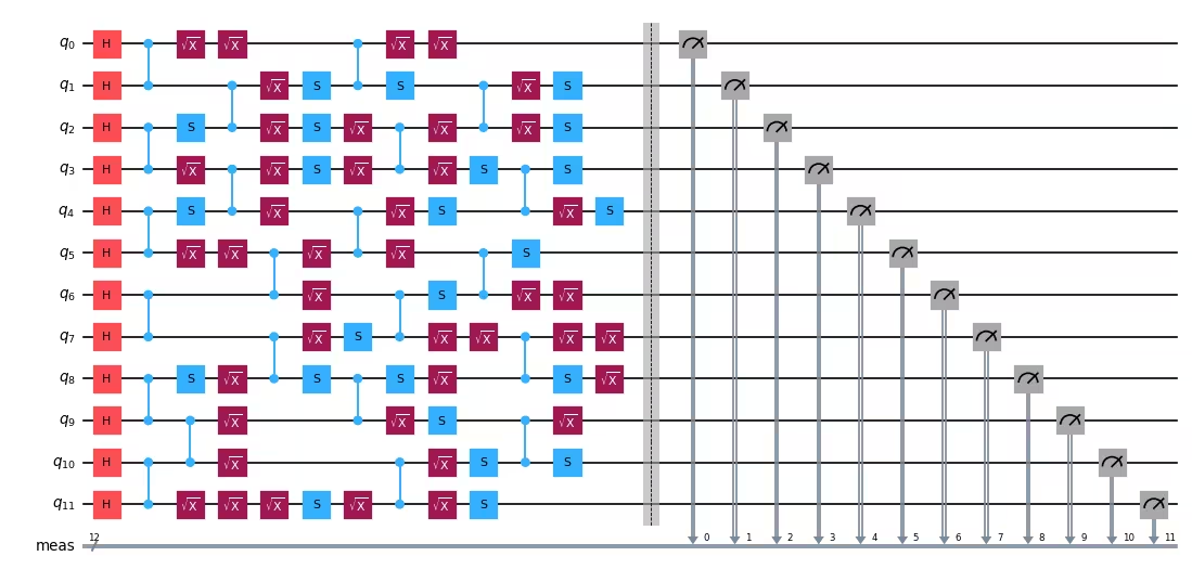
The payload circuit is a shallow one-dimensional brickwork random Clifford circuit. Because the circuit is Clifford, it prepares a stabilizer state whose fidelity you can estimate directly from sampled stabilizer expectation values. Start with a shallow circuit so that the checks are easy to visualize in the next step.
num_qubits = 12
depth = 4
seed = 1764
rng = np.random.default_rng(seed)
np.random.seed(seed)

circuit = random_clifford_circuit(num_qubits, depth, rng)
circuit.measure_all()
circuit.draw("mpl", fold=-1, scale=0.6)
Output:
Step 2: Optimize for quantum hardware execution
Mapping the circuit to hardware sets the physical qubit layout, the noise model that scores candidate checks, and the checks themselves.
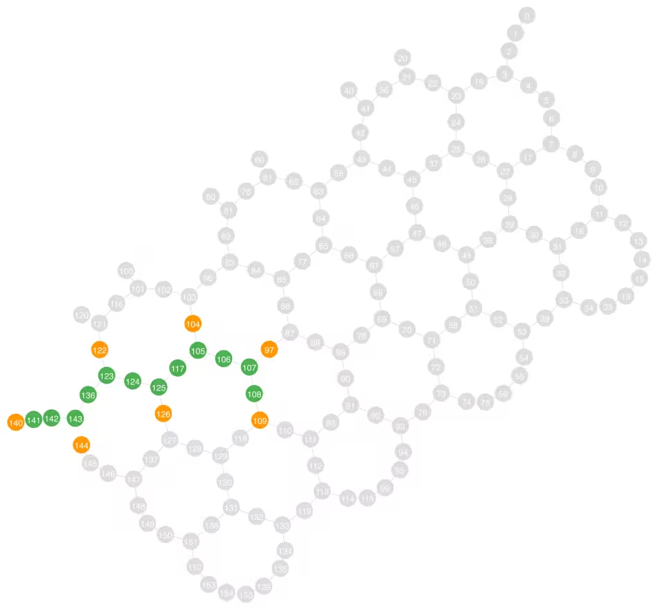
First, select a backend and search its coupling map for a one-dimensional qubit layout with the find_check_layout helper defined in the Setup section. The helper builds random self-avoiding walks that avoid the highest-error gates and readouts, and it keeps the path that offers the most target and ancilla pairs. Because the search reads the connectivity and error data from the backend itself, the same code runs on any IBM Quantum QPU. The get_check_qubits function then returns the target and ancilla pairs, where a check on target_qubits[i] uses ancilla_qubits[i].
In the coupling graph that follows, the green qubits are payload qubits and the orange qubits are the ancillas that implement the checks. Qubits with an adjacent ancilla are used as target qubits for checks.
service = QiskitRuntimeService()
backend = service.least_busy(operational=True, simulator=False)

print(f"Backend: {backend.name}")

# Search for a low-error path, then pair each target qubit with a neighboring ancilla
layout = find_check_layout(backend, num_qubits, rng)
target_qubits, ancilla_qubits = get_check_qubits(backend, layout)
num_checks = len(target_qubits)

print(f"Target qubits:  {target_qubits}")
print(f"Ancilla qubits: {ancilla_qubits}")
plot_coupling_map(
    num_qubits=backend.num_qubits,
    qubit_coordinates=getattr(
        backend.configuration(), "qubit_coordinates", None
    ),
    coupling_map=backend.configuration().coupling_map,
    figsize=(12, 12),
    qubit_color=[
        "#4CAF50"
        if i in set(layout)
        else "#FF9800"
        if i in set(ancilla_qubits)
        else "#DDDDDD"
        for i in backend.coupling_map.graph.node_indices()
    ],
    qubit_size=220,
    line_width=2,
    font_size=90,
)
Output:
Backend: ibm_boston
Target qubits:  [105, 107, 108, 123, 125, 141, 143]
Ancilla qubits: [104, 97, 109, 122, 126, 140, 144]
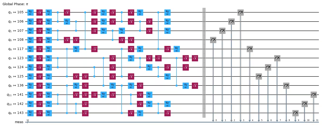
With the backend and layout chosen, transpile the payload into an instruction set architecture (ISA) circuit. It is only necessary to set the layout and translate the gates into the native gate set of the backend.
pm = generate_preset_pass_manager(
    optimization_level=0, backend=backend, initial_layout=layout
)
circuit_isa = pm.run(circuit)
circuit_isa.draw("mpl", fold=-1, scale=0.6)
Output:
Next, model how the gate and readout noise on the backend affects execution. The noise model determines where in the circuit a check captures the most error. A more accurate model improves the detection, but it is usually not necessary to learn one by sampling the QPU. The model that follows infers a uniform depolarizing channel for gate and readout noise from qiskit-ibm-runtime benchmark data.
noise_model = NoiseModel.from_backend(
    backend, layout, uniform_gate_noise=True
)
print(noise_model)
Output:
NoiseModel(gate_noise=0.001079865281450939, readout_noise=0.006001790364583333, idling_noise=None)
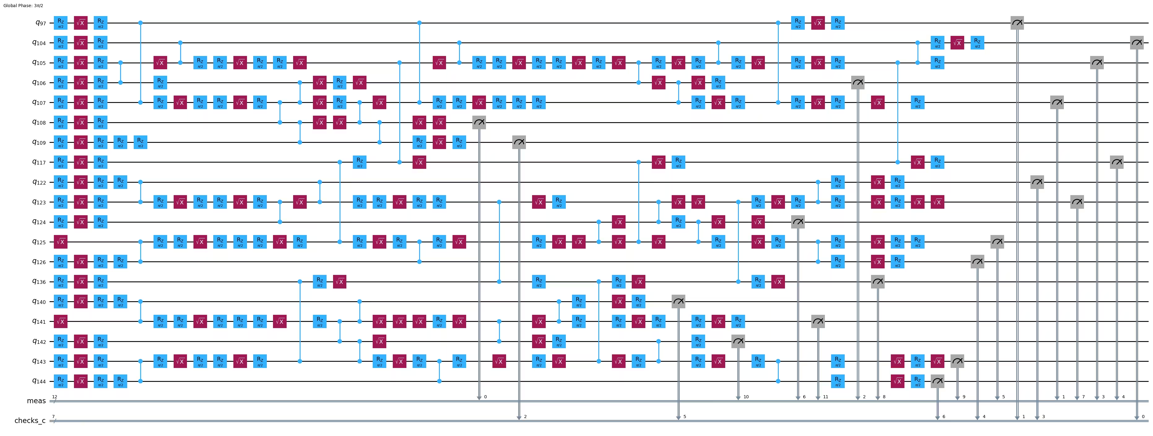
Now add checks to the circuit. The add_pauli_checks function takes the Clifford payload, the list of target qubits, and the noise model. The ancilla_qubits argument tells the function which physical ancilla to pair with each target. Checks are added in the order the target qubits appear, so the final layout of the checked circuit is layout + ancilla_qubits. To run an output circuit with fewer (i) checks, the final layout is layout + ancilla_qubits[:i].
The output of add_pauli_checks is a sequence of circuits with an increasing number of checks, from no checks up to one check on every target qubit. The visualization confirms that the checks use the specified target and ancilla pairs. For details on finding good checks, see Sections II to IV of the supplementary information in reference [1].
checked = add_pauli_checks(
    circuit_isa,
    target_qubits,
    noise_model,
    ancilla_qubits=ancilla_qubits,
    cost="gamma",
    method="windowed",
    seed=seed,
)

print(f"Physical layout of payload and ancillas: {layout + ancilla_qubits}")
print("Checked circuit:")
checked[-1].circuit.draw("mpl", fold=-1, idle_wires=False)
Output:
Physical layout of payload and ancillas: [108, 107, 106, 105, 117, 125, 124, 123, 136, 143, 142, 141, 104, 97, 109, 122, 126, 140, 144]
Checked circuit:
Step 3: Execute using Qiskit primitives
To make the effect of gate noise visible, increase the depth of the payload and sample a subset of its stabilizers. Each stabilizer is generally not qubit-wise commuting with the others, so a single set of checks is not valid for two different stabilizers. Rather than group stabilizers into commuting sets, find a good set of checks for each stabilizer independently. Sampling stabilizers uniformly at random gives an unbiased fidelity estimate.
Build the deeper circuit and draw a random sample of its stabilizers.
depth = 24
num_stabilizers = 20
num_shots = 1_000

circuit = random_clifford_circuit(num_qubits, depth, rng)

# Build the full stabilizer group, then sample from it uniformly at random
circ_no_meas = circuit.remove_final_measurements(inplace=False)
stabilizer_group = PauliList([Pauli("I" * num_qubits)])
for generator in (
    Pauli(label) for label in Clifford(circ_no_meas).to_labels(mode="S")
):
    stabilizer_group = stabilizer_group + stabilizer_group.compose(generator)

keep = np.where(
    stabilizer_group.x.any(axis=1) | stabilizer_group.z.any(axis=1)
)[0]
chosen = np.random.default_rng(seed).choice(
    keep, size=min(num_stabilizers, len(keep)), replace=False
)
stabilizers = [stabilizer_group[int(i)] for i in chosen]

two_qubit_depth = circuit.depth(lambda x: x.operation.num_qubits == 2)
print(
    f"Sampled {len(stabilizers)} stabilizers of a {circuit.num_qubits}-qubit "
    f"circuit with two-qubit depth {two_qubit_depth}: "
    f"{{{stabilizers[0]}, {stabilizers[1]}, ...}}"
)
Output:
Sampled 20 stabilizers of a 12-qubit circuit with two-qubit depth 24: {ZXIIXZYYXIZZ, XXXYIIZYXIII, ...}
For each sampled stabilizer, rotate the circuit so that the stabilizer is measured in the computational basis, transpile it onto the backend, and find a good set of checks. The target and ancilla pairs are shuffled together for each stabilizer so that each target keeps its ancilla. Remember that checks are committed sequentially in the order the target qubits are given, and a committed check is not changed as more checks are added.
noisy_circuits = []
checked_circuits = []
depths_2q = []
t0 = time.time()
for i, pauli in enumerate(tqdm(stabilizers)):
    noisy_circuits.append(pm.run(append_basis_rotation(circuit, pauli)))
    # Shuffle target and ancilla pairs together so each target keeps its ancilla
    targets, ancillas = zip(
        *random.sample(
            list(zip(target_qubits, ancilla_qubits, strict=True)),
            k=len(target_qubits),
        ),
        strict=True,
    )
    checked_circuits.append(
        add_pauli_checks(
            noisy_circuits[-1],
            list(targets),
            noise_model,
            ancilla_qubits=list(ancillas),
            cost="gamma",
            method="windowed",
            seed=seed + 1 + i,
        )
    )
    depths_2q.append(
        checked_circuits[-1][-1].circuit.depth(lambda x: len(x.qubits) == 2)
    )

print(
    f"Added {num_checks} checks to {len(stabilizers)} circuits "
    f"in {(time.time() - t0):.0f}s."
)
print(
    f"On average, two-qubit depth increased from "
    f"{circuit.depth(lambda x: len(x.qubits) == 2)} to {int(np.mean(depths_2q))} "
    f"when adding {num_checks} checks."
)
Output:
100%|██████████| 20/20 [00:15<00:00, 1.29it/s]
Added 7 checks to 20 circuits in 15s.
On average, two-qubit depth increased from 24 to 33 when adding 7 checks.
Sample the bare payload and the checked circuits with Qiskit Aer. The simulator uses the same depolarizing model that scored the checks, so the noise that the checks target is the noise that the simulator applies.
aer_nm = AerNoiseModel()
aer_nm.add_all_qubit_quantum_error(
    depolarizing_error(noise_model.gate_noise, 2), ["cz"]
)
p = noise_model.readout_noise
aer_nm.add_all_qubit_readout_error(ReadoutError([[1 - p, p], [p, 1 - p]]))
noisy_sim = AerSimulator(method="stabilizer", noise_model=aer_nm)

counts = []
for i, checked_circ_result in enumerate(tqdm(checked_circuits)):
    noisy_counts = (
        noisy_sim.run(
            noisy_circuits[i], shots=num_shots, seed_simulator=seed * i + 1
        )
        .result()
        .get_counts()
    )
    checked_counts_per_variant = []
    for k, ck in enumerate(checked_circ_result):
        variant_counts = (
            noisy_sim.run(
                ck.circuit, shots=num_shots, seed_simulator=seed * i + 2 + k
            )
            .result()
            .get_counts()
        )
        checked_counts_per_variant.append(variant_counts)
    counts.append((noisy_counts, checked_counts_per_variant))
Output:
100%|██████████| 20/20 [00:17<00:00, 1.13it/s]
Step 4: Post-process and return result in desired classical format
Each check uses entangling gates between one ancilla and one target. The ancilla starts in , so stabilizes its input. Propagating forward through the checked circuit yields a Pauli operator on the output whose non-identity terms define the check's support. A check passes when the bits in its support have even parity. A sample is kept only when every check passes.
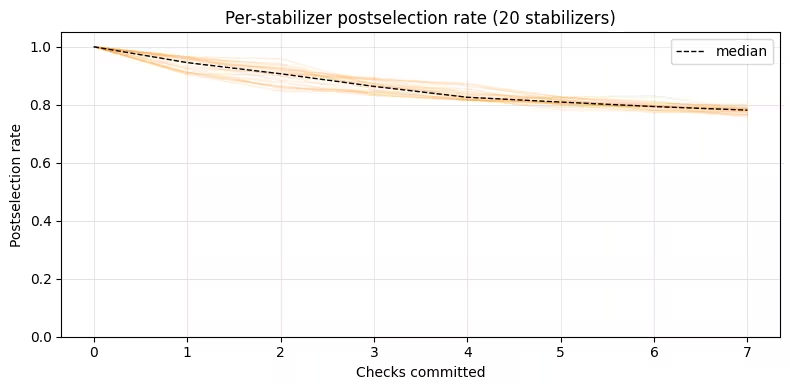
The get_postselection_method of each CheckedCircuit returns a function that maps a measured bitstring to a syndrome vector. Keep the samples whose syndrome is zero for every check, and discard the rest. The chart that follows shows that adding more checks lowers the postselection rate. A lower postselection rate needs more shots to reach a target accuracy, so there is a tradeoff between detection capability and sampling cost. The rate appears to converge, which indicates that additional checks contribute less detection capability.
rate_per_variant = []
kept_per_stab = []
for i, (_, checked_counts_per_variant) in enumerate(counts):
    rates = []
    kept_at_num_checks = None
    for k, variant_counts in enumerate(checked_counts_per_variant):
        ps_fn = checked_circuits[i][k].get_postselection_method()
        kept = {
            bs: n for bs, n in variant_counts.items() if not ps_fn(bs).any()
        }
        rates.append(sum(kept.values()) / num_shots)
        if k == num_checks:
            kept_at_num_checks = kept
    rate_per_variant.append(rates)
    kept_per_stab.append(kept_at_num_checks)

max_len = max(len(s) for s in rate_per_variant)
rates_arr = np.full((len(rate_per_variant), max_len), np.nan)
for i, s in enumerate(rate_per_variant):
    rates_arr[i, : len(s)] = s
ks = np.arange(max_len)

fig, ax = plt.subplots(figsize=(8, 4))
ax.plot(ks, rates_arr.T, color="#ff8c00", alpha=0.15, linewidth=1)
ax.plot(
    ks,
    np.nanmedian(rates_arr, axis=0),
    color="black",
    linewidth=1,
    linestyle="--",
    label="median",
)
ax.set_xlabel("Checks committed")
ax.set_ylabel("Postselection rate")
ax.set_ylim((0, 1.05))
ax.set_title(
    f"Per-stabilizer postselection rate ({len(rates_arr)} stabilizers)"
)
ax.legend()
ax.grid(True, alpha=0.3)
plt.tight_layout()
plt.show()
Output:
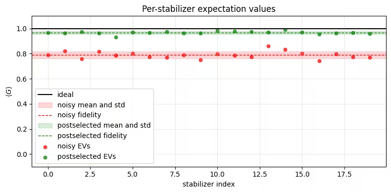
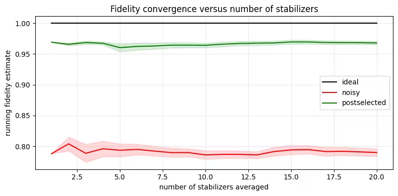
Now compare the fidelity of the bare noisy state with the postselected state. Postselecting only the samples with no detected error raises the expectation value of every stabilizer, and therefore the estimated fidelity. The postselected values use fewer samples than the raw values, yet the expectation values are more accurate and the sampled variance is lower. Notice also that the mean postselection rate is close to the noisy fidelity. This is what you expect when the checks detect nearly all erroneous samples: the fraction of samples that pass every check approaches the fraction of error-free samples, which is the fidelity of the noisy state.
results = []
for i, ((noisy_counts, _), kept) in enumerate(
    zip(counts, kept_per_stab, strict=True)
):
    results.append(
        (
            expectation(noisy_counts, stabilizers[i]),
            expectation(kept, stabilizers[i]),
            sum(kept.values()) / num_shots,
        )
    )

fidelity_noisy = float(np.nanmean([r[0] for r in results]))
fidelity_postsel = float(np.nanmean([r[1] for r in results]))
psr = float(np.mean([r[2] for r in results]))
print(
    f"ideal fidelity:          1.0\n"
    f"noisy fidelity:          {fidelity_noisy:.4f}\n"
    f"postselected fidelity:   {fidelity_postsel:.4f}\n"
    f"mean postselection rate: {psr:.3f}"
)

evs_ideal = np.ones(len(results))
evs_noisy = np.array([r[0] for r in results])
evs_post = np.array([r[1] for r in results])
idx = np.arange(len(results))


def strip(ax, ys, color, label):
    m, s = np.nanmean(ys), np.nanstd(ys)
    ax.axhspan(
        m - s, m + s, color=color, alpha=0.15, label=f"{label} mean and std"
    )
    ax.axhline(
        m, color=color, linewidth=1, linestyle="--", label=f"{label} fidelity"
    )


fig, ax = plt.subplots(figsize=(8, 4))
ax.axhline(np.nanmean(evs_ideal), color="black", linewidth=1.5, label="ideal")
strip(ax, evs_noisy, "red", "noisy")
strip(ax, evs_post, "green", "postselected")
ax.scatter(idx, evs_noisy, color="red", s=22, alpha=0.7, label="noisy EVs")
ax.scatter(
    idx,
    evs_post,
    color="green",
    s=22,
    alpha=0.7,
    label="postselected EVs",
)
ax.set_xlabel("stabilizer index")
ax.set_ylabel(r"$\langle G \rangle$")
ax.set_ylim((-0.1, 1.1))
ax.set_title("Per-stabilizer expectation values")
ax.legend(loc="lower left")
ax.grid(True, alpha=0.3)
plt.tight_layout()
plt.show()

M = np.arange(1, len(results) + 1)
fig, ax = plt.subplots(figsize=(8, 4))
for ys, color, label in [
    (evs_ideal, "black", "ideal"),
    (evs_noisy, "red", "noisy"),
    (evs_post, "green", "postselected"),
]:
    cm, sem = cum_mean_sem(ys)
    ax.plot(M, cm, color=color, linewidth=1.5, label=label)
    ax.fill_between(M, cm - sem, cm + sem, color=color, alpha=0.15)
ax.set_xlabel("number of stabilizers averaged")
ax.set_ylabel("running fidelity estimate")
ax.set_title("Fidelity convergence versus number of stabilizers")
ax.legend()
ax.grid(True, alpha=0.3)
plt.tight_layout()
plt.show()
Output:
ideal fidelity:          1.0
noisy fidelity:          0.7899
postselected fidelity:   0.9679
mean postselection rate: 0.780
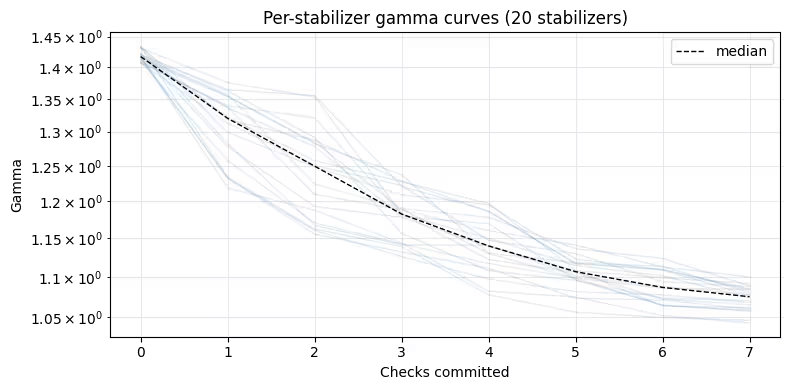
The gamma score reports how much of the modeled noise channel remains undetected by the checks. Plotting the gamma score against the number of committed checks shows how the detection capability improves as each check is added. A value of 1.0 means that the checks capture all of the modeled noise. The curves fall toward 1.0 as more checks are committed, which shows that each additional check captures part of the remaining undetected error.
stab_scores = [
    [variant.cost for variant in checked_circ_result]
    for checked_circ_result in checked_circuits
]
max_len = max(len(s) for s in stab_scores)
scores = np.full((len(stab_scores), max_len), np.nan)
for i, s in enumerate(stab_scores):
    scores[i, : len(s)] = s
ks = np.arange(max_len)

fig, ax = plt.subplots(figsize=(8, 4))
ax.plot(ks, scores.T, color="#4682b4", alpha=0.15, linewidth=1)
ax.plot(
    ks,
    np.nanmedian(scores, axis=0),
    color="black",
    linewidth=1,
    linestyle="--",
    label="median",
)
ax.set_xlabel("Checks committed")
ax.set_ylabel("Gamma")
ax.set_yscale("log")
ax.set_title(f"Per-stabilizer gamma curves ({len(scores)} stabilizers)")
ax.legend()
ax.grid(True, alpha=0.3, which="both")
plt.tight_layout()
plt.show()
Output:
Large-scale hardware example
The same workflow runs on hardware with a larger, deeper payload. This section reuses the backend from the simulator example but builds a new 20-qubit layout with its own target and ancilla pairs and pass manager, then submits the circuits to the QPU in a single job. At this size, most shots trigger at least one check, so the postselection rate is low, and each circuit needs a large shot budget for enough samples to survive. The example therefore concentrates its budget on a few sampled stabilizers; this is still an unbiased fidelity estimate, but is coarser than the simulator example's average over many stabilizers.
One thing changes relative to the simulator example: instead of inferring a uniform depolarizing channel from calibration data, this section learns the noise model with NoiseLearner and builds the qiskit-paulice model from the result with NoiseModel.from_pauli_lindblad_maps. A learned Pauli-Lindblad model captures the spatial structure of the noise on this specific layout, rather than assuming every edge is equally noisy, so the check placement is scored against noise more similar to that affecting the QPU. Learning the noise requires sampling the QPU and should be accounted for in any overall QPU sampling budget.
The parameters that follow set the number of qubits, the depth, the number of stabilizers, and the number of shots. Scale hw_num_shots with the inverse of the postselection rate: at a 3% rate, 40,000 shots leave roughly 1,200 postselected samples per circuit. Increase hw_num_stabilizers for a more precise fidelity estimate at the cost of more circuits per job, each of which needs the same shot budget.
Steps 1-4 (compressed into a single code block)
The following cell runs the same four steps as the simulator example. It builds the larger payload and samples a few stabilizers (step 1); chooses a layout, learns the noise model on it, and finds the fully checked circuit for each stabilizer (step 2); submits one Sampler job that contains both the bare and the checked circuits (step 3); and postselects the checked counts to compare the noisy and postselected fidelity estimates, per stabilizer and on average (step 4). At this size, enumerating the full stabilizer group like the simulator example is infeasible, so the cell subsamples a random subset of stabilizers to calculate an estimate of the fidelity.
Note that step 2 does more here than in the simulator example: learning the noise model submits its own NoiseLearner job before the Sampler job, so the cell runs two jobs in total. They carry the tags TUT_ASPC_LEARN and TUT_ASPC so that you can find them later. See Organize and search by job tags for more on tagging jobs.
# -------------------------Step 1: build a larger payload and sample stabilizers-------------------------
hw_num_qubits = 20
hw_depth = 36
hw_num_stabilizers = 10
hw_num_shots = 40_000

hw_circuit = random_clifford_circuit(hw_num_qubits, hw_depth, rng)
hw_no_meas = hw_circuit.remove_final_measurements(inplace=False)

# Enumerating all 2^n stabilizers is infeasible at this size, so draw each
# stabilizer by composing a random subset of the group generators
hw_generators = [
    Pauli(label) for label in Clifford(hw_no_meas).to_labels(mode="S")
]
sample_rng = np.random.default_rng(seed)
hw_stabilizers = []
while len(hw_stabilizers) < hw_num_stabilizers:
    mask = sample_rng.integers(0, 2, hw_num_qubits).astype(bool)
    if not mask.any():
        continue  # skip the identity
    stabilizer = Pauli("I" * hw_num_qubits)
    for generator, chosen in zip(hw_generators, mask, strict=True):
        if chosen:
            stabilizer = stabilizer.compose(generator)
    hw_stabilizers.append(stabilizer)

# -------------------------Step 2: find a 20-qubit layout, learn its noise, and add checks-------------------------
# A single bad coupler or bad-readout qubit on the path drags every
# stabilizer down, so search harder and with tighter error thresholds
hw_layout = find_check_layout(
    backend,
    hw_num_qubits,
    rng,
    num_trials=500,
    max_gate_error=0.015,
    max_readout_error=0.05,
)
hw_target_qubits, hw_ancilla_qubits = get_check_qubits(backend, hw_layout)
hw_pm = generate_preset_pass_manager(
    optimization_level=0, backend=backend, initial_layout=hw_layout
)
print(f"Layout with {len(hw_target_qubits)} check pairs: {hw_layout}")

# ----- learn a Pauli-Lindblad noise model on this layout -----
# The simulator example scored checks against a uniform depolarizing channel
# inferred from calibration data. Here, learn the noise instead: NoiseLearner
# runs its own job on the QPU and returns a Pauli-Lindblad channel per unique
# entangling layer, so the checks are placed against the noise this layout
# actually has, including its spatial structure. All the sampled stabilizers
# share the same entangling layers and differ only in their final basis
# rotation, so learning on the bare payload covers all of them.
learner = NoiseLearner(
    mode=backend,
    options={
        "max_layers_to_learn": 4,
        "num_randomizations": 32,
        "shots_per_randomization": 128,
        "environment": {"job_tags": ["TUT_ASPC_LEARN"]},
    },
)
learner_job = learner.run([hw_pm.run(hw_circuit)])
print(f"Submitted noise-learner job {learner_job.job_id()}")
hw_layer_errors = learner_job.result().data

# To see how much the learned model helps, swap the next line for the
# simulator example's uniform model - a one-line change:
# hw_noise_model = NoiseModel.from_backend(backend, hw_layout, uniform_gate_noise=True)
hw_noise_model = learned_noise_model(hw_layer_errors, hw_layout)
# NoiseLearner characterizes gate noise only, so keep the readout estimate
# from calibration data rather than leaving it unset
hw_noise_model.readout_noise = NoiseModel.from_backend(
    backend, hw_layout, uniform_gate_noise=True
).readout_noise
print(
    f"Learned {len(hw_layer_errors)} layers; "
    f"readout noise {hw_noise_model.readout_noise:.5f}"
)

# ----- add the fully checked circuit per stabilizer -----
hw_noisy_circuits = []
hw_checked_circuits = []
for i, pauli in enumerate(tqdm(hw_stabilizers)):
    bare = hw_pm.run(append_basis_rotation(hw_circuit, pauli))
    hw_noisy_circuits.append(bare)
    variants = add_pauli_checks(
        bare,
        hw_target_qubits,
        hw_noise_model,
        ancilla_qubits=hw_ancilla_qubits,
        cost="gamma",
        method="windowed",
        seed=seed + 1 + i,
    )
    hw_checked_circuits.append(variants[-1])  # keep the fully checked circuit

# -------------------------Step 3: submit one Sampler job with the bare and checked circuits-------------------------
sampler = Sampler(mode=backend)
sampler.options.default_shots = hw_num_shots
sampler.options.environment.job_tags = ["TUT_ASPC"]

pubs = hw_noisy_circuits + [cc.circuit for cc in hw_checked_circuits]
job = sampler.run(pubs)
print(f"Submitted job {job.job_id()} with {len(pubs)} circuits")

# -------------------------Step 4: postselect and compare fidelity-------------------------
result = job.result()
n_stab = len(hw_stabilizers)

hw_results = []
for i in range(n_stab):
    noisy_counts = result[i].join_data().get_counts()
    checked_counts = result[n_stab + i].join_data().get_counts()
    ps_fn = hw_checked_circuits[i].get_postselection_method()
    kept = {bs: c for bs, c in checked_counts.items() if not ps_fn(bs).any()}
    hw_results.append(
        (
            expectation(noisy_counts, hw_stabilizers[i]),
            expectation(kept, hw_stabilizers[i]),
            sum(kept.values()) / sum(checked_counts.values()),
        )
    )

hw_fidelity_noisy = float(np.nanmean([r[0] for r in hw_results]))
hw_fidelity_postsel = float(np.nanmean([r[1] for r in hw_results]))
hw_psr = float(np.mean([r[2] for r in hw_results]))
print(
    f"noisy fidelity estimate:        {hw_fidelity_noisy:.4f}\n"
    f"postselected fidelity estimate: {hw_fidelity_postsel:.4f}\n"
    f"mean postselection rate:        {hw_psr:.4f} "
    f"(~{int(round(hw_psr * hw_num_shots))} kept shots per circuit)"
)

# Per-stabilizer breakdown. The postselection rate varies from stabilizer to
# stabilizer, so a stabilizer whose postselected value barely moves is usually
# one whose checks rejected little; the kept-shot count says how much of the
# gap is statistics rather than signal.
print("\nper-stabilizer results:")
print(
    f"{'idx':>3}  {'noisy':>8}  {'postsel':>8}  {'psr':>7}  {'kept shots':>10}"
)
for i, (noisy, post, psr_i) in enumerate(hw_results):
    print(
        f"{i:>3}  {noisy:>8.4f}  {post:>8.4f}  {psr_i:>7.4f}  "
        f"{int(round(psr_i * hw_num_shots)):>10}"
    )

hw_noisy = np.array([r[0] for r in hw_results])
hw_post = np.array([r[1] for r in hw_results])
idx = np.arange(n_stab)

fig, ax = plt.subplots(figsize=(9, 4))
ax.axhline(1.0, color="black", linewidth=1.5, label="ideal")
strip(ax, hw_noisy, "red", "noisy")
strip(ax, hw_post, "green", "postselected")
ax.scatter(idx, hw_noisy, color="red", s=22, alpha=0.7, label="noisy EVs")
ax.scatter(
    idx,
    hw_post,
    color="green",
    s=22,
    alpha=0.7,
    label="postselected EVs",
)
ax.set_xlabel("stabilizer index")
ax.set_ylabel(r"$\langle G \rangle$")
ax.set_ylim((-0.1, 1.1))
ax.set_xticks(idx)
ax.set_title("Per-stabilizer expectation values on hardware")
# Outside the axes so it cannot hide a data point
ax.legend(loc="center left", bbox_to_anchor=(1.02, 0.5), frameon=False)
ax.grid(True, alpha=0.3)
plt.tight_layout()
plt.show()
Output:
Layout with 11 check pairs: [153, 152, 151, 138, 131, 130, 129, 118, 109, 110, 111, 98, 91, 90, 89, 78, 69, 70, 71, 58]
Submitted noise-learner job d9f4mncjeosc73fjfmkg
Learned 4 layers; readout noise 0.00470
100%|██████████| 10/10 [01:01<00:00, 6.18s/it]
Submitted job d9f4s04jeosc73fjftkg with 20 circuits
noisy fidelity estimate:        0.3685
postselected fidelity estimate: 0.6869
mean postselection rate:        0.2851 (~11404 kept shots per circuit)

per-stabilizer results:
idx     noisy   postsel      psr  kept shots
  0    0.3769    0.6918   0.3247       12987
  1    0.3745    0.6760   0.2999       11995
  2    0.3659    0.6389   0.3549       14196
  3    0.3821    0.7060   0.2660       10641
  4    0.3653    0.7475   0.2531       10124
  5    0.3752    0.7022   0.2698       10791
  6    0.3508    0.7144   0.2711       10842
  7    0.3485    0.7087   0.2381        9523
  8    0.3825    0.6289   0.2928       11711
  9    0.3630    0.6549   0.2808       11232
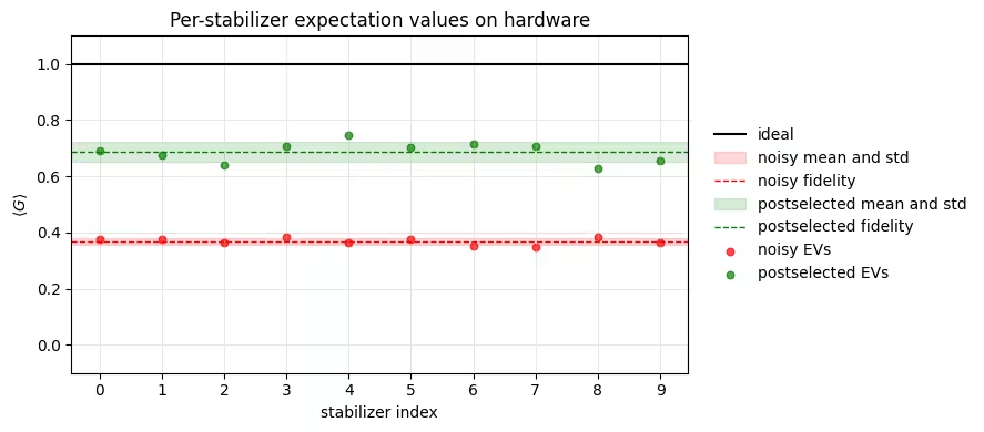
For circuits of this size, most samples contain at least one detected error, so the postselection rate is small and postselection discards most shots. The samples that pass every check give a much better expectation value than the bare circuit, and the per-stabilizer values separate cleanly from the noisy baseline. To tighten the fidelity estimate, sample more stabilizers with the same per-circuit shot budget. To raise the postselection rate, reduce the circuit depth or commit fewer checks; to push to larger payloads, scale the shot budget with the inverse of the postselection rate.
Next steps
If you found this work interesting, you might be interested in the following material:
- The tutorial on repetition codes for an introduction to quantum error correction.
- The
qiskit-paulicedocumentation for the full check-finding API, and the package's GitHub repository for the source code. - The paper Low-overhead error detection with spacetime codes for the theory behind the checks.
References
- [1] Martiel, S., & Javadi-Abhari, A. (2025). Low-overhead error detection with spacetime codes. arXiv preprint arXiv:2504.15725.
- [2] van den Berg, E., Bravyi, S., Gambetta, J. M., Jurcevic, P., Maslov, D., & Temme, K. (2023). Single-shot error mitigation by coherent Pauli checks. Physical Review Research, 5(3), 033193.