Probabilistic error cancellation with shaded lightcones

Usage estimate: 10 minutes on an IBM Heron processor (NOTE: This is an estimate only. Your runtime might vary.)

Learning outcomes

After going through this tutorial, users should understand:

• What probabilistic error cancellation (PEC) is, and why its sampling overhead $\gamma^2$ grows exponentially with the total noise acting on the circuit
• How shaded lightcones (SLC) bound each noise term's contribution to the target observable, letting you spend the mitigation budget where it matters and trade a bounded residual bias for lower sampling overhead
• How to learn layer noise with NoiseLearnerV3 and inject anti-noise through samplomatic and the Executor
• How to combine PEC and PEC+SLC with TREX and post-selection to estimate an expectation value on hardware

Prerequisites

We suggest that users are familiar with the following topics before going through this tutorial:

• The Qiskit patterns workflow
• Using the Estimator primitive to calculate expectation values of an observable
• Error mitigation techniques such as Pauli twirling and TREX, covered in Combine error mitigation options with the Estimator primitive

Background

This tutorial demonstrates how to mitigate errors by using the shaded lightcone (SLC) addon. This addon is an evolution of the probabilistic error cancellation (PEC) technique, wherein a user learns the noise of unique layers in a circuit and then cancels out the noise by applying single-qubit gates and post-processing techniques. Compared to other methods, PEC offers more robust bounds on the bias of the mitigated result, but tends to suffer from a higher overhead in terms of QPU time. During PEC, to compensate for attenuation of the expectation value by noise, the average result is rescaled by a factor of $\gamma = \exp(\sum_{l,\sigma} 2\lambda_{l,\sigma})$, where $\lambda_{l,\sigma}$ is the learned noise rate of error Pauli $\sigma$ at layer $l$ in the circuit. This rescaling increases the variance by a factor of $\gamma^2$, and thus also multiplies the number of circuit executions needed on the QPU by $\gamma^2$, which we call the sampling cost or sampling overhead. Because $\gamma$ grows exponentially, PEC is often limited to shallow or few-qubit circuits. Learn more about PEC in Probabilistic error cancellation with sparse Pauli-Lindblad models on noisy quantum processors.

If we can identify errors that do not need to be mitigated, we can decrease this sampling cost exponentially. A first step in this direction is implementing locally aware error mitigation, which uses a quickly computable conventional "lightcone" to reduce the PEC overhead by bounding an observable's sensitivity to errors throughout the circuit, extending the feasibility of PEC to larger scales for some problems. Errors outside of this lightcone cannot affect the measured outcome and can therefore be excluded from the error cancellation procedure. This exclusion decreases the sampling overhead, in some cases substantially, without introducing additional bias. In particular, for measuring a local observable $O$ of a fixed-depth circuit, the required sampling overhead eventually plateaus when scaling the number of qubits in the circuit (see Fig. 2b in Locality and error mitigation of quantum circuits).

Shaded lightcones (SLC) go further, using classical simulations to more tightly bound the sensitivity to errors throughout the circuit. This trades some QPU time for CPU time and reduces the sampling overhead needed to renormalize the bias. Instead of a hard cutoff, each potential error in the circuit is assigned a graded "shade" that upper-bounds the susceptibility of the observable to that error. This refined characterization allows for more efficient, targeted applications of PEC with reduced variance, while giving the user the ability to controllably tune the bias in the observable estimation. See Lightcone shading for classically accelerated quantum error mitigation for more details.

Our workflow for the SLC addon leverages the samplomatic library together with the QuantumProgram and Executor classes added to Qiskit Runtime in qiskit-ibm-runtime 0.47.0, allowing users to have more modular control of execution settings for error suppression and mitigation while retaining ease of use.

SLC error-mitigation workflow at a glance

For modeling the QPU's noise, we use a sparse Pauli-Lindblad noise model with one- and two-qubit Pauli error rates, locally generated on each qubit and edge of the device. With this choice, the SLC error-mitigation workflow presented in this tutorial is as follows:

a. CPU — Bound per-error impact of one- and two-qubit Pauli errors

1. Forward propagation (bound effect on observable). Propagate each error to the end of the circuit and compute its commutator with the observable.
   • Truncate operator terms during evolution to keep computation tractable.
   • Further tighten these bounds by a loose back-propagation of the observable based on quantum speed limits.
2. Backward propagation (bound effect on initial state). Propagate each error to the start of the circuit and compute its commutator with the initial state.

b. QPU — Learn noise rates. Use NoiseLearnerV3 to estimate rates of the Pauli-Lindblad noise model.

c. CPU — Prioritize mitigation

1. Update merged bounds with learned noise rates. Combine forward and backward bounds that were previously computed and update them with learned noise rates.
2. Rank noise components to mitigate by using the computed bounds and learned rates. Prioritize each possible noise error based on its estimated impact on bias and the associated expense to correct.

d. QPU — Insert antinoise and run. Execute the circuit of interest with antinoise (inverse noise) specified by using Box annotations.

e. CPU — Estimate observable. Compute the expectation value, applying measurement-based post-selection to reduce non-Markovian noise impact.

Noise learning overview

Noise learning is a common step in several error-mitigation methods, carried out by the noise learner; it also appears in the probabilistic error amplification tutorial. In NoiseLearnerV3, a user can specifically identify the to-be-learned noise layers as CircuitInstruction objects, which allows users to compute the desired SLC noise bounds for each layer in the manner described above. The learned Pauli-Lindblad model provides coefficients to be used in the PEC+SLC prioritization. The way in which the gates are collected into layers can be determined by using the generate_boxing_pass_manager and find_unique_box_instructions convenience functions, and then fed into the SLC utility function generate_noise_model_paulis, as described in Step 2 below.

Part 1	Part 2	Part 3
Pauli-twirl two-qubit gate layers	Repeat identity pairs of layers and learn noise	Derive a fidelity (error for each noise channel)

Post-processing overview

After executing on quantum hardware by using the samplomatic and Executor framework, we convert our bitstring measurements into the desired observable value. In the case of our mirrored Ising circuit, we will ideally get a measured observable of 1, as all qubits should ideally return to their starting point of $|0\rangle$. When computing the observable value with the executor_expectation_values function, we apply a few post-processing techniques that reduce noise impact. These include removing shots affected by non-Markovian noise, readout-error mitigation, and accounting for details of our PEC implementation. Details are discussed in Step 4 below.

Requirements

Before starting this tutorial, be sure you have the following installed:

• Qiskit SDK v2.2 or later, with visualization support (pip install 'qiskit[visualization]')
• Qiskit Runtime v0.47 or later (pip install qiskit-ibm-runtime)
• Shaded lightcone Qiskit addon 0.1 or later (pip install qiskit-addon-slc)
• Qiskit addon utils 0.3 or later (pip install 'qiskit-addon-utils')
• Samplomatic v0.13 or later (pip install samplomatic)

Setup

First, import the packages and functions needed to run this notebook.

from multiprocessing import set_start_method

# Setting this value prevents itertools.starmap deadlock on UNIX systems
set_start_method("spawn")

# Needed to prevent PySCF from parallelizing internally (SLC only)
%set_env OMP_NUM_THREADS=1

Output:

env: OMP_NUM_THREADS=1

import numpy as np
from matplotlib import pyplot as plt

from qiskit import QuantumCircuit
from qiskit.quantum_info import SparsePauliOp
from qiskit.transpiler import generate_preset_pass_manager, PassManager

from qiskit_ibm_runtime import (
    QiskitRuntimeService,
    QuantumProgram,
    Executor,
    NoiseLearnerV3,
)

import samplomatic
from samplomatic.utils import find_unique_box_instructions, get_annotation
from samplomatic.annotations import InjectNoise
from samplomatic.transpiler import generate_boxing_pass_manager

from qiskit_addon_utils.exp_vals.measurement_bases import (
    get_measurement_bases,
)
from qiskit_addon_utils.exp_vals.expectation_values import (
    executor_expectation_values,
)
from qiskit_addon_utils.noise_management import (
    gamma_from_noisy_boxes,
    trex_factors,
)
from qiskit_addon_utils.noise_management.post_selection import PostSelector
from qiskit_addon_utils.noise_management.post_selection.transpiler.passes import (
    AddPostSelectionMeasures,
    AddSpectatorMeasures,
)

from qiskit_addon_slc.bounds import (
    compute_backward_bounds,
    compute_forward_bounds,
    compute_local_scales,
    merge_bounds,
    tighten_with_speed_limit,
)
from qiskit_addon_slc.utils import (
    generate_noise_model_paulis,
    map_modifier_ref_to_ref,
)
from qiskit_addon_slc.visualization import draw_shaded_lightcone

Small-scale simulator example

Like other learning-based error mitigation methods, PEC with shaded lightcones mitigates the physical noise of a specific quantum processor, so it depends on hardware services with no meaningful analog on an ideal simulator:

• NoiseLearnerV3 experimentally characterizes the sparse Pauli-Lindblad noise channel on each unique two-qubit layer. On a noiseless simulator there is no noise to cancel.
• The Executor primitive samples the twirled, anti-noise-injected circuits generated by samplomatic on a backend.

The shaded-lightcone bound computation is classical, but it is only meaningful relative to the learned hardware noise rates, which set the mitigation budget and sampling overhead. For these reasons we skip the small-scale simulator example and demonstrate the full PEC+SLC workflow directly on hardware, with each step of the Qiskit pattern broken out below.

Large-scale hardware example

We run the complete PEC+SLC workflow on a 20-qubit mirrored Ising circuit executed on IBM Quantum® hardware, following the four steps of a Qiskit pattern.

Step 1: Map the problem

For ease of demonstration, we select a 1D mirror Ising chain. The 1D Ising chain gives a nicely dense circuit structure, which is convenient for showcasing PEC implementations. A mirror circuit makes it straightforward to know the expected outcome (namely, we should measure an observable of 1).

Because we run a mirror circuit, for every gate in the second half of the circuit there is an inverse gate in the first half. As the measured observable $\langle X_6 Z_{13}\rangle$ has non-Z-basis measurements, and the executor accounts for the desired basis at the end of the circuit, we provide a prepare_basis function that inserts the appropriate gates at the start of the mirror circuit. This detail is specific to our mirror-circuit demonstration. The get_measurement_bases function lets us identify which gates are needed and where to append them, while keeping track of qubit-index subtleties arising from box annotation conventions, as discussed in the section on preparing canonical basis measurements.

num_qubits = 20
target_obs_sparse = [("XZ", [6, 13], 1.0)]

observable = SparsePauliOp.from_sparse_list(
    target_obs_sparse, num_qubits=num_qubits
)

bases_virt, reverser_virt = get_measurement_bases(observable)

num_trotter_steps = 10
rx_angle = np.pi / 4

def construct_ising_circuit(
    num_qubits: int,
    num_trotter_steps: int,
    rx_angle: float,
    barrier: bool = True,
) -> QuantumCircuit:
    circuit = QuantumCircuit(num_qubits)

    for step in range(num_trotter_steps):
        circuit.rx(rx_angle, range(num_qubits))
        if barrier:
            circuit.barrier()
        for first_qubit in (1, 2):
            for idx in range(first_qubit, num_qubits, 2):
                # equivalent to Rzz(-pi/2):
                circuit.sdg([idx - 1, idx])
                circuit.cz(idx - 1, idx)
        if barrier:
            circuit.barrier()

    return circuit


def prepare_basis(
    circuit: QuantumCircuit, basis: list[int]
) -> QuantumCircuit:
    # basis is a list of integer values from 0 to 3. These map to the basis measurement as:
    # 0 = I; 1 = Z; 2 = X; 3 = Y
    assert len(basis) == circuit.num_qubits

    out_circ = circuit.copy_empty_like()
    for qb, bas in enumerate(basis):
        if bas in {0, 1}:
            continue
        if bas == 2:
            out_circ.h(qb)
        elif bas == 3:
            out_circ.rx(-np.pi / 2, qb)

    out_circ.barrier()
    out_circ.compose(circuit, inplace=True)
    return out_circ


def mirror_circuit(
    circuit: QuantumCircuit, *, inverse_first: bool = False
) -> QuantumCircuit:
    mirror_circ = circuit.copy_empty_like()
    mirror_circ.compose(
        circuit.inverse() if inverse_first else circuit, inplace=True
    )
    mirror_circ.barrier()
    mirror_circ.compose(
        circuit if inverse_first else circuit.inverse(), inplace=True
    )
    mirror_circ.measure_active()
    return mirror_circ

# Instantiate circuit
circuit = construct_ising_circuit(
    num_qubits, num_trotter_steps, rx_angle, barrier=False
)
mirrored_circuit = mirror_circuit(circuit, inverse_first=True)
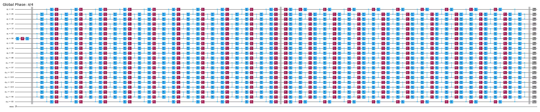
mirrored_circuit = prepare_basis(mirrored_circuit, bases_virt[0])

mirrored_circuit.draw(
    "mpl", fold=-1, scale=0.3, idle_wires=False, measure_arrows=False
)

Output:

Step 2: Optimize

We will optimize details associated with the circuit to be run, the observable to be measured, and the noise-learning parameters. As a starting point, we instantiate a backend with fractional gates turned on. These fractional gates allow for greater sensitivity in some of our post-selection filtering.

# Initialize the Qiskit Runtime service using your saved credentials
service = QiskitRuntimeService()

# Fractional gates allow greater sensitivity in some of our post-selection filtering
backend = service.backend("ibm_boston", use_fractional_gates=True)
print(f"Using backend: {backend.name}")

Output:

Using backend: ibm_boston

First, we will transpile our circuit to ISA instructions, as required for execution on our QPUs. For the data collected in this experiment, we hand select our qubits based on evaluation of the highest quality chain.

layout = [
    44,
    45,
    46,
    47,
    57,
    67,
    68,
    69,
    78,
    89,
    88,
    87,
    97,
    107,
    106,
    105,
    104,
    103,
    96,
    83,
]

isa_pm = generate_preset_pass_manager(
    backend=backend, initial_layout=layout, optimization_level=0
)

isa_circuit = isa_pm.run(mirrored_circuit)
assert isa_circuit.layout.final_index_layout() == layout

isa_observable = observable.apply_layout(
    layout, num_qubits=isa_circuit.num_qubits
)

wire_order = layout + [
    q for q in range(isa_circuit.num_qubits) if q not in layout
]
isa_circuit.draw(
    "mpl",
    fold=-1,
    scale=0.3,
    idle_wires=False,
    wire_order=wire_order,
    measure_arrows=False,
)

Output:

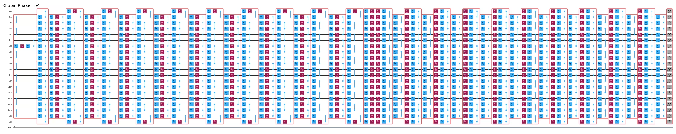
Box the circuit

For ease of implementation, we will utilize the generate_boxing_pass_manager transpilation pass, which places the circuit instructions into annotated boxes. These boxes clearly indicate where, in the case of PEC, antinoise should be injected into the circuit. For details on settings, refer to the Samplomatic documentation.

Note that the SLC workflow requires the use of inject_noise_strategy="individual_modification" later in the process because this allows us to uniquely identify each BoxOp in the circuit.

The find_unique_box_instructions function iterates through the provided boxed circuit and identifies those that have unique 2Q layers or measurements, for the purpose of noise learning and noise injection.

# Box circuit with Twirl and InjectNoise annotations
boxes_pm = generate_boxing_pass_manager(
    twirling_strategy="active",
    inject_noise_strategy="individual_modification",
    inject_noise_targets="gates",
    measure_annotations="all",
)


boxed_circuit = boxes_pm.run(isa_circuit)

# Find the unique instructions (layers) from boxed circuit
unique_2q_instructions = find_unique_box_instructions(
    boxed_circuit, normalize_annotations=None, undress_boxes=True
)

boxed_circuit.draw(
    "mpl",
    fold=-1,
    scale=0.3,
    idle_wires=False,
    wire_order=wire_order,
    measure_arrows=False,
)

Output:

Prepare canonical bases measurements

Due to how the qubits are labeled when identifying unique 2Q layers, one must take special care to keep track of qubit ordering. Below, we introduce the notion of canonical_qubits as a means to appropriately update the qubit ordering when providing it to the executor, as a result of how qubit order is captured when boxing circuits and finding unique instructions. See the Qubit ordering convention documentation for details.

# Determine the canonical qubits order
meas_box = boxed_circuit.data[-1]
canonical_qubits = [
    idx
    for idx, qubit in enumerate(boxed_circuit.qubits)
    if qubit in meas_box.qubits
]

# map canonical qubit to physical (isa) qubit
c_2_p = {c: p for c, p in enumerate(canonical_qubits)}
# map physical (isa) qubit to virtual qubit (index in original circuit)
p_2_v = {p: v for v, p in enumerate(layout)}
# compute map between virtual and canonical qubit indices.
c_2_v = {c: p_2_v[p] for c, p in c_2_p.items()}

assert len(c_2_v) == num_qubits

bases_canon = [
    np.array([base_i[c_2_v[c]] for c in range(num_qubits)], dtype=np.uint8)
    for base_i in bases_virt
]

Workflow for lightcone shading, noise learning, and anti-noise injection

Note: In this tutorial, we run the SLC bound computations before the noise learning completes, so the to-be-mitigated circuit is run as close in time as possible to the learned noise model. In principle this workflow can be parallelized further: a noise-learning job can run while, in parallel, the noise bounds are estimated. For an arbitrary quantum circuit the noise-bound computation can scale with a weakly exponential dependence, so parallelizing the bound computation (for example, across many CPU cores) yields tighter bounds for a given compute-time budget, and the QPU executions and bound computations can themselves be parallelized for the most efficient workflow.

Predict to-be-learned noise-model Paulis

The generate_noise_model_paulis function goes through each boxed layer of the provided circuit and generates all relevant weight-one and weight-two Pauli terms, taking into account the circuit's qubit connectivity, and selecting terms that are relevant to the active nodes and edges. These terms are then used to compute forward and backward noise bounds.

noise_model_paulis = generate_noise_model_paulis(
    unique_2q_instructions, backend.coupling_map, boxed_circuit
)

noise_model_rates = {ref: None for ref in noise_model_paulis}

a. Compute and tighten forward bounds

The compute_forward_bounds function evaluates the commutation relations between the gates in each layer and the above-generated Pauli terms in terms of how forward-propagation errors affect the desired observable $A$. For gates that commute with the Pauli terms, nothing is done. For Clifford gates, they are pushed toward the beginning of the circuit. For non-Clifford gates, we approximate their influence on the target observables to later be prioritized for noise cancellation (after all bounds have been merged). This bound is achieved by first applying the L2 norm (namely, the square root of the sum of squares of the relevant Pauli-term coefficients). When there are too many qubit terms involved, we revert to a looser bound that uses the triangle inequality.

Set the bound-computation parameters

slc_atol = 1e-8
slc_eigval_max_qubits = 18
slc_evolution_max_terms = 1000
slc_num_processes = 8
slc_timeout = 60

forward_bounds = compute_forward_bounds(
    boxed_circuit,
    noise_model_paulis,
    isa_observable,
    evolution_max_terms=slc_evolution_max_terms,
    eigval_max_qubits=slc_eigval_max_qubits,
    atol=slc_atol,
    num_processes=slc_num_processes,
    timeout=slc_timeout,
)

Output:

Bounds computation timed out.

Visualize the SLC for manual inspection

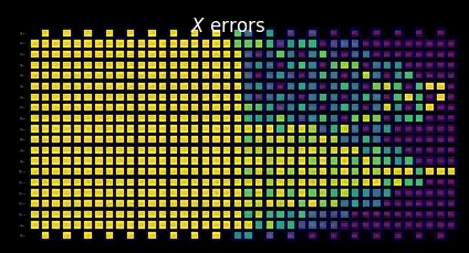
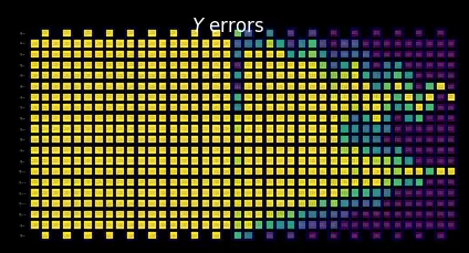
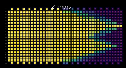
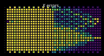
You can interpret the behavior of the shaded bounds by examining how the measurements and Pauli terms interact with the local errors. These patterns are characteristic of this kicked Ising Hamiltonian time-evolution problem and also appear in the paper Lightcone Shading for Classically Accelerated Quantum Error Mitigation, with several telltale features:

• We can clearly distinguish the two cones arising from the two non-identity Paulis in the observable.
• We can see that the X measurement on qubit 6 commutes with the X error in the rightmost layer.
• We can see that the Z Pauli on qubit 13 commutes with the Z error in the rightmost layer.
• When we reach the timeout specified above, the remaining layers to the left are filled entirely with trivial bounds of two.

for p in "XYZ":
    display(
        draw_shaded_lightcone(
            boxed_circuit,
            forward_bounds,
            noise_model_paulis,
            pauli_filter=p,
            scale=0.15,
            fold=-1,
            idle_wires=False,
            wire_order=wire_order,
            measure_arrows=False,
        )
    )

Output:

b. Compute and tighten forward bounds

We next tighten the bounds by using the tighten_with_speed_limit function, which tracks how the observable spreads backward through the circuit and uses that spread to place upper bounds on the effect of each noise operator, taking the smaller of the forward bound just computed, and the backward-propagation bound.

forward_bounds_tighter = tighten_with_speed_limit(
    forward_bounds, boxed_circuit, noise_model_paulis, isa_observable
)

Visualize the SLC for manual inspection

We can further tighten the bounds by accounting for lightcone limitation. In principle, this gives us a smoother transition from the computed bounds to the trivial bounds set forth after the timeout was reached. Here, the effect is not as visible because the lightcones have already reached the edge of the circuit.

for p in "XYZ":
    display(
        draw_shaded_lightcone(
            boxed_circuit,
            forward_bounds_tighter,
            noise_model_paulis,
            pauli_filter=p,
            scale=0.15,
            fold=-1,
            idle_wires=False,
            wire_order=wire_order,
            measure_arrows=False,
        )
    )

Output:

c. Compute backward bounds

This part of noise prediction evaluates how an error at a particular layer can affect the input state $\rho$. The compute_backward_bounds function first inverts the circuit, removes measurement gates, and then proceeds with a similar analysis as was done for the forward-bound computations.

backward_bounds = compute_backward_bounds(
    boxed_circuit,
    noise_model_paulis,
    evolution_max_terms=slc_evolution_max_terms,
    num_processes=slc_num_processes,
    timeout=slc_timeout,
)

Visualize the SLC for manual inspection

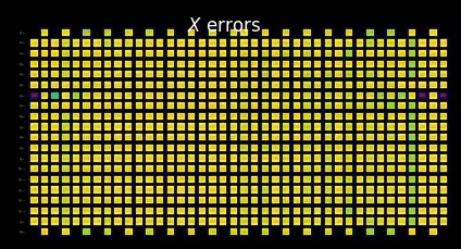
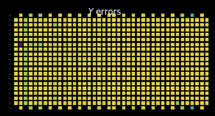
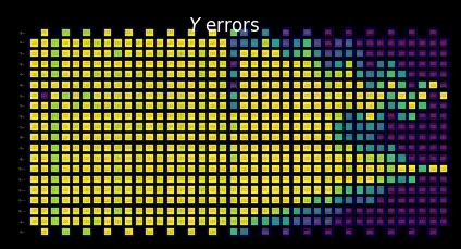
From computing backward bounds, we can see how the initial state structure governs the early behavior of error propagation:

• We can clearly see how the Z errors initially commute with the |0⟩ initial state.
• Only on qubit 6, where we initialize the +1 eigenstate of the X basis, does a Z error fail to commute, while an X error does commute.

for p in "XYZ":
    display(
        draw_shaded_lightcone(
            boxed_circuit,
            backward_bounds,
            noise_model_paulis,
            pauli_filter=p,
            scale=0.15,
            fold=-1,
            idle_wires=False,
            wire_order=wire_order,
            measure_arrows=False,
        )
    )

Output:

Preview merged bounds without learned noise rates

The merged_bounds function determines the point in the circuit where switching from backward bounds to forward bounds minimizes the total estimated bias on the desired observable. This bias is computed as the sum of the backward-bound contributions for all noise locations before that point, plus the forward-bound contributions for all noise locations after it. Currently, this is done uniformly for all qubits.

Important Note: The point to switch from forward to backward bounds depends on the learned noise rates.

merged_bounds = merge_bounds(
    boxed_circuit,
    forward_bounds_tighter,
    backward_bounds,
    noise_model_rates,
)

Output:

Missing noise rates. Partitioning backward/forward commutator bounds by assuming uniform error rates.
Optimal spacetime partitioning not implemented!Just partitioning list of noisy boxes.

Visualize the SLC for manual inspection

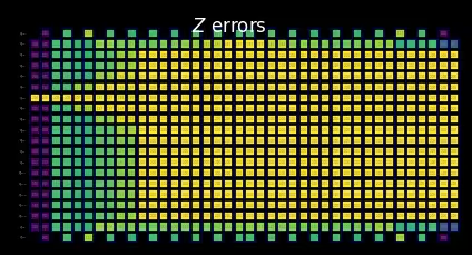
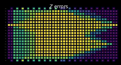
After merging the backward and tightened forward bounds, the behavior of the combined SLCs becomes clear:

• The function above tells us that a partition is chosen at which the switch from backward to tightened forward bounds takes place.
• We can see below that the SLCs now contain partial backward and partial tightened forward bounds.

for p in "XYZ":
    display(
        draw_shaded_lightcone(
            boxed_circuit,
            merged_bounds,
            noise_model_paulis,
            pauli_filter=p,
            scale=0.15,
            fold=-1,
            idle_wires=False,
            wire_order=wire_order,
            measure_arrows=False,
        )
    )

Output:

Step 3: Execute

In this section we begin the part of the workflow that uses a real quantum device. For this learning-based error mitigation method, there are two steps:

1. Learn the noise by using NoiseLearnerV3.
2. Execute an error-mitigation circuit with the samplomatic and Executor framework.

With the bounded errors from our quantum circuit, we learn the associated noise rates to prioritize our error budget, determine the sampling overhead, and execute on a QPU.

a. Learn the noise rates

The noise learner characterizes the noise processes affecting the gates in one or more circuits of interest, based on the sparse Pauli-Lindblad noise model. The run() method launches a noise-learning job for the provided unique two-qubit layers, using the options specified in the noise-learner configuration. These options control the Pauli-twirling strategy, the number of randomizations and shots, the learning depths, and post-selection.

We also choose the learning depths deliberately. A practical finding for learning-based mitigation with samplomatic is that it is highly beneficial for the deepest learning depth to match the depth of the circuit you want to mitigate. Because NLv3 layer_pair_depths are measured in layer pairs (a layer plus its inverse), we set the deepest value to half the circuit's two-qubit-layer depth.

post_selection_enabled = True

# Match the deepest noise-learning depth to the depth of the circuit being
# mitigated. NLv3 ``layer_pair_depths`` are measured in layer pairs (a layer
# plus its inverse), so the deepest value is half the circuit's two-qubit-layer
# depth. Learning to this depth markedly improves the quality of the mitigation.
num_2q_layers = sum(
    get_annotation(inst.operation, InjectNoise) is not None
    for inst in boxed_circuit.data
)
max_layer_pair_depth = num_2q_layers // 2
layer_pair_depths = sorted({1, 2, 4, 8, 12, 16, max_layer_pair_depth})

noise_learner_options = {
    "num_randomizations": 64,
    "shots_per_randomization": 128,
    "layer_pair_depths": layer_pair_depths,
    "post_selection": {
        "enable": post_selection_enabled,
        "strategy": "edge",
        "x_pulse_type": "rx",
    },
    "environment": {"job_tags": ["TUT_SLC"]},
}

noise_learner = NoiseLearnerV3(backend, noise_learner_options)

noise_learner_job = noise_learner.run(unique_2q_instructions)

noise_learner_result = noise_learner_job.result()

if post_selection_enabled:
    print(
        "Minimum fraction of shots kept for noise learning experiments: ",
        end="",
    )
    print(
        f"{min([min(d.values()) for d in [nlr.metadata['post_selection']['fraction_kept'] for nlr in noise_learner_result[:2]]]):.2f}"
    )

Output:

Minimum fraction of shots kept for noise learning experiments: 0.85

# Get a dict mapping each InjectNoise.ref to its learned PauliLindbladMap
refs_2_plm = noise_learner_result.to_dict(
    unique_2q_instructions, require_refs=False
)

b.i. Update merged bounds with actual learned noise rates

Now that the specific noise model has been learned, we can apply the learned noise rates to the predicted noise bounds and obtain a final determination of which bounds have the most impact on minimizing the bias.

merged_bounds = merge_bounds(
    boxed_circuit,
    forward_bounds_tighter,
    backward_bounds,
    refs_2_plm,
)

Output:

Optimal spacetime partitioning not implemented!Just partitioning list of noisy boxes.

b.ii. Compute the local_scales for the hardware execution

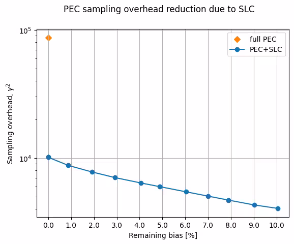
compute_local_scales looks at each possible noise error in the circuit and estimates how much that error could bias the final measurement, as well as how expensive it would be to correct it. It then ranks the errors by how worthwhile they are to mitigate and selects the subset that reduces bias as much as possible, while staying within the allowed sampling-cost budget (or achieving a desired accuracy). The result is a set of scaling factors indicating which errors will be actively mitigated and which will be left unmitigated (local_scales), along with the predicted total sampling cost overhead (sampling_costs) and remaining bias (residual_bias_bound).

The ability to control the desired remaining bias is a critical feature of the SLC implementation of PEC. Whereas in the original implementation, the sampling overhead always targeted zero bias, we can tune the required sampling overhead with a trade-off in the expected remaining bias. This helps let the user stay within a fixed sampling budget, which can be particularly useful when initially prototyping a workflow.

id_map = map_modifier_ref_to_ref(boxed_circuit)

summed_rates = 0.0
for box_id, noise_id in id_map.items():
    learned_plm = refs_2_plm[noise_id]
    summed_rates += np.sum(learned_plm.rates)
    # print(f"{box_id}:\tgamma = {np.exp(2 * summed_rates):1.6e}\tsampling cost = {np.exp(4 * summed_rates):1.6e}")
total_gamma = np.exp(2 * summed_rates)
print(
    f"Full PEC gamma={total_gamma}, sampling cost (gamma^2) = {total_gamma**2}"
)

Output:

Full PEC gamma=294.94827441509057, sampling cost (gamma^2) = 86994.48458043957

biases = []
costs = []
for bias in [0.0] + np.arange(0.001, 0.102, 0.01).tolist():
    _, cost_, bias_ = compute_local_scales(
        boxed_circuit,
        merged_bounds,
        refs_2_plm,
        sampling_cost_budget=np.inf,
        bias_tolerance=bias,
    )
    biases.append(bias_)
    costs.append(cost_)

Trade off sampling overhead against residual bias

xticks = np.arange(0, 11)

fig, ax = plt.subplots()
ax.scatter(
    [0], [total_gamma**2], marker="D", c="tab:orange", label="full PEC"
)
ax.plot(
    100 * np.array(biases),
    np.array(costs),
    "o-",
    c="tab:blue",
    label="PEC+SLC",
)
ax.set_yscale("log")
ax.set_xticks(xticks, [f"{x:.1f}" for x in xticks])

ax.set_xlabel("Remaining bias [%]")
ax.set_ylabel(r"Sampling overhead, $\gamma^2$")
ax.grid()
ax.legend()
fig.suptitle("PEC sampling overhead reduction due to SLC")

Output:

Text(0.5, 0.98, 'PEC sampling overhead reduction due to SLC')

chosen_bias_thres = 0.1

local_scales, sampling_cost, residual_bias_bound = compute_local_scales(
    boxed_circuit,
    merged_bounds,
    refs_2_plm,
    sampling_cost_budget=np.inf,
    bias_tolerance=chosen_bias_thres,
)
print(
    f"PEC+SLC sampling cost (gamma^2) = {sampling_cost} "
    f"w/ remaining bias = {100 * residual_bias_bound:.1f}%"
)

Output:

PEC+SLC sampling cost (gamma^2) = 4200.504852399781 w/ remaining bias = 9.4%

c. Execute the circuit of interest with antinoise

c.i. Prepare template circuit by using samplex

The samplex is an output of the build method of Samplomatic, which encodes all the information that is required to generate randomized parameters for template_circuit. These are then used to set up the QuantumProgram objects, which are in turn run on a QPU with the Executor primitive. Each QuantumProgram can contain several items, which you can think of as a pair of template and samplex.

See the Hello samplomatic tutorial for details.

# Build template circuit and samplex for later use with the "Executor"
template_circuit, samplex = samplomatic.build(boxed_circuit)

# Set up postselection if it's been enabled
if post_selection_enabled:
    # Set up post selection PM (to add PS instructions)
    post_selection_pm = PassManager(
        [
            AddSpectatorMeasures(backend.coupling_map),
            AddPostSelectionMeasures(x_pulse_type="rx"),
        ]
    )
    final_template_circuit = post_selection_pm.run(template_circuit)
else:
    final_template_circuit = template_circuit

c.ii. Set up the QuantumProgram

num_randomizations = 4096
shots_per_randomization = 64
chunk_size = 256

# Set up QuantumProgram
program = QuantumProgram(shots=shots_per_randomization, noise_maps=refs_2_plm)

# no EM

# Collect up a dict of the other arguments that need to be bound to samplex_inputs
samplex_inputs = {
    f"noise_scales.{ref}": float(0) for ref in local_scales.keys()
}
samplex_inputs |= {"basis_changes": {"basis0": bases_canon[0]}}

# Convert samplex_inputs into a dict to pass to QuantumProgram
samplex_arguments = (
    samplex.inputs().bind(**samplex_inputs).make_broadcastable()
)

program.append_samplex_item(
    circuit=final_template_circuit,
    samplex=samplex,
    samplex_arguments=samplex_arguments,
    shape=(num_randomizations,),
    chunk_size=chunk_size,
)

# plain PEC

# Collect a dict of the other arguments that need to be bound to samplex_inputs
samplex_inputs = {
    f"noise_scales.{ref}": float(-1) for ref in local_scales.keys()
}
samplex_inputs |= {"basis_changes": {"basis0": bases_canon[0]}}

# Convert samplex_inputs into a dict to pass to QuantumProgram
samplex_arguments = (
    samplex.inputs().bind(**samplex_inputs).make_broadcastable()
)

program.append_samplex_item(
    circuit=final_template_circuit,
    samplex=samplex,
    samplex_arguments=samplex_arguments,
    shape=(num_randomizations,),
    chunk_size=chunk_size,
)

# PEC+SLC

# Collect a dict of the other arguments that need to be bound to samplex_inputs
samplex_inputs = {
    f"noise_scales.{ref}": float(-1) for ref in local_scales.keys()
}
samplex_inputs |= {"basis_changes": {"basis0": bases_canon[0]}}
samplex_inputs |= {"local_scales": local_scales}

# Convert samplex_inputs into a dict to pass to QuantumProgram
samplex_arguments = (
    samplex.inputs().bind(**samplex_inputs).make_broadcastable()
)

program.append_samplex_item(
    circuit=final_template_circuit,
    samplex=samplex,
    samplex_arguments=samplex_arguments,
    shape=(num_randomizations,),
    chunk_size=chunk_size,
)

c.iii. Execute program with the Executor primitive

executor = Executor(backend)

job_exec = executor.run(program)

results_exec = job_exec.result()

Step 4: Post-process

As we calculate the final expectation value of interest by using executor_expectation_values, we implement a few post-processing techniques to help ensure we obtain the highest-quality results possible. First, we apply our twirled readout error extinction (TREX), which accounts for any errors occurring during the readout process. Then, we fix errors due to non-Markovian noise on our Heron backends by using a post-selection method. This method measures active and spectator qubits, then applies a slow rotation to each qubit, and then measures again. In instances where the two measurements do not confirm a flipped qubit as expected, these shots are discarded by applying a mask from the PostSelector. Within the mask computation, a specific strategy can be set to filter based on single-qubit nodes or neighboring spectator edges, which can influence both the number of shots filtered out and the quality of the results.

measurement_noise_map = noise_learner_result[2].to_pauli_lindblad_map()
trex_scale_factors = trex_factors(measurement_noise_map, reverser_virt)

post_selection_strategy = "node"

def post_process_conv(datum, steps=16, gamma=None, ps=False, trex=False):
    meas = datum["meas"]
    flips = datum["measurement_flips.meas"]
    signs = datum.get("pauli_signs", None)

    meas_basis_axis = None
    avg_axis = 0

    mask = None
    if ps and post_selection_enabled:
        # Post-select the results
        post_selector = PostSelector.from_circuit(
            circuit=final_template_circuit, coupling_map=backend.coupling_map
        )

        # Compute the ps mask for filtering results
        mask = post_selector.compute_mask(
            datum, strategy=post_selection_strategy
        )

        # Compute fraction of shots kept from post selection
        total_num_shots = num_randomizations * shots_per_randomization
        ps_ratio = np.sum(mask) * 100 / total_num_shots / len(bases_canon)
        print(
            f"With {post_selection_strategy}-based post selection ({ps_ratio:.1f}% of shots kept):"
        )

    results = []
    for i in range(steps, num_randomizations + 1, steps):
        # Compute mitigated expvals w/out post-selection
        res = executor_expectation_values(
            meas[:i],
            reverser_virt,
            meas_basis_axis,
            avg_axis=avg_axis,
            measurement_flips=flips[:i],
            pauli_signs=signs[:i] if signs is not None else None,
            postselect_mask=mask[:i] if mask is not None else None,
            rescale_factors=trex_scale_factors if trex else None,
            gamma_factor=gamma,
        )
        results.append(res[0])
    return results

gamma_pec = gamma_from_noisy_boxes(refs_2_plm, id_map)
gamma_slc = gamma_from_noisy_boxes(refs_2_plm, id_map, local_scales)

steps = 16

results = {}

for label, result_idx, gamma, use_ps, use_trex in [
    ("PEC", 1, gamma_pec, True, True),
    ("PEC+SLC", 2, gamma_slc, True, True),
    ("Unmitigated", 0, None, False, False),
]:
    res = post_process_conv(
        results_exec[result_idx],
        steps=steps,
        gamma=gamma,
        ps=use_ps,
        trex=use_trex,
    )
    results[label] = res

Output:

With node-based post selection (26.7% of shots kept):
With node-based post selection (26.8% of shots kept):

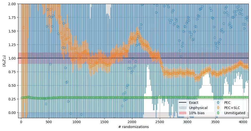
From examination of the experimental results, we can directly compare the behavior of the different approaches: PEC, PEC combined with SLC, and the unmitigated baseline. Some specific details to highlight:

• The unmitigated result sits far outside the 10% bias band (near 0.3) and is unaffected by the number of randomizations.
• On this device, full PEC carries an enormous sampling overhead ($\gamma^2 \approx 8.7\times10^4$). At that cost it cannot converge within the randomizations used: the plain-PEC estimates stay wildly scattered with large error bars across the full range.
• SLC reduces the overhead roughly 20-fold (to $\gamma^2 \approx 4.2\times10^3$, for a residual-bias bound of about 9%). PEC+SLC consequently behaves far better than plain PEC: its error bars are much smaller and contract steadily as randomizations accumulate, and its estimate settles into the physical region and converges close to the exact value of 1, approaching the 10% bias band from just below. The contrast with plain PEC — which remains scattered across nearly the entire plot — clearly demonstrates the benefit of lightcone shading.
• The error bars also shrink faster for PEC+SLC than for plain PEC.

fig, ax = plt.subplots(1, 1, figsize=(12, 6))

ax.axhline(1.0, color="black", label="Exact")
ax.fill_between(
    [-50, 4100], -10, 0, color="grey", alpha=0.25, label="Unphysical"
)
ax.fill_between([-50, 4100], 1, 10, color="grey", alpha=0.25)
ax.fill_between(
    [-50, 4100], 0.9, 1.1, color="red", alpha=0.25, label="10% bias"
)

for label, res in results.items():
    ax.errorbar(
        list(range(steps, num_randomizations + 1, steps)),
        [r[0] for r in res],
        yerr=[r[1] for r in res],
        alpha=0.75,
        marker="o",
        linestyle="",
        markerfacecolor="none",
        label=label,
    )

ax.set_ylabel(r"$\langle X_{6}Z_{13}\rangle$")
ax.set_xlabel("# randomizations")
ax.grid()

ax.legend(ncols=2)
ax.set_ylim([-0.1, 2.0])
ax.set_xlim([-50, 4100])

Output:

(-50.0, 4100.0)

Next steps

If you found this work interesting, you might be interested in the following material: