Improving expectation values with propagated noise absorption (PNA)

Usage estimate: 10 minutes on an IBM Heron processor (NOTE: This is an estimate only. Your runtime might vary.)

Learning outcomes

After going through this tutorial, users should understand:

• What propagated noise absorption (PNA) is, and how it mitigates two-qubit gate noise by absorbing learned inverse noise channels into the measured observable
• How to use samplomatic to box and annotate circuit layers for twirling, basis changes, and noise injection
• How to learn layer noise with NoiseLearnerV3 and propagate it into a noise-mitigating observable with qiskit-addon-pna
• How to sample randomized circuits with the QuantumProgram and Executor classes in Qiskit Runtime, and combine PNA with TREX and post-selection

Prerequisites

We suggest that users are familiar with the following topics before going through this tutorial:

• The Qiskit patterns workflow
• Using the Estimator primitive to calculate expectation values of an observable
• Error mitigation techniques such as Pauli twirling and TREX, covered in Combine error mitigation options with the Estimator primitive

Background

In this tutorial, we demonstrate how to leverage advanced error-mitigation tools in Qiskit to improve expectation value estimation in noisy quantum experiments.

What is propagated noise absorption (PNA)?

Propagated noise absorption is a technique for mitigating gate errors by propagating the observable through the inverse noise channel affecting two-qubit gates, resulting in a noise-mitigating observable.

Quantum error mitigation enables us to extract useful expectation values from noisy quantum hardware without requiring full fault tolerance. PNA specifically focuses on absorbing noise effects into the observable itself rather than modifying the circuit operations.

Each noisy gate in a quantum circuit can be modeled as an ideal gate followed by a noise channel. PNA learns or characterizes these noise channels and defines their inverses. Instead of inserting the inverse operations into the hardware execution (which is typically infeasible), PNA propagates the inverse noise channels forward through the circuit and applies them to the observable. This process transforms the observable $O$ into a new operator $\tilde{O}$, such that measuring $\tilde{O}$ on the noisy circuit yields the same expectation value as measuring $O$ on an ideal, noise-free circuit.

This can be summarized as:

1. Model each noisy gate $u_i$ as an ideal operation followed by a noise channel $\Lambda_i$.
2. Learn or estimate each $\Lambda_i$ using noise characterization tools.
3. Define and propagate the inverse noise maps $\Lambda_i^{-1}$ forward through the circuit using Pauli transfer techniques.
4. Absorb these inverses into the observable, resulting in a noise-mitigated operator $\tilde{O}$.

When the noise is described as a Pauli channel (or more generally as a sparse Pauli-Lindblad channel), this propagation can be performed efficiently using Pauli propagation. Pauli propagation provides a framework for approximating how inverse noise channels transform as they pass through layers of Clifford and non-Clifford operations, while controlling the computational complexity.

By shifting the mitigation into the observable, PNA avoids the large sampling overhead that would otherwise come from inserting physical correction operations into the circuit. Instead, the original noisy circuit is executed, while the observable is transformed into a new operator $\tilde{O}$ whose expectation value cancels the effects of noise.

Visualizing the PNA workflow

The process can be understood through the following conceptual stages. The first schematic illustrates a standard noisy experiment.

If we learn the noise model, we can apply its inverse and cancel the noise.

Instead of implementing the inverse noise channel by sampling it on the QPU as in probabilistic error cancellation (PEC), we apply it classically to the measured observable using Pauli propagation. The resulting observable effectively mitigates the learned gate noise when measured.

Modular error mitigation with samplomatic and the Executor

The PNA approach builds upon a modular error-mitigation architecture in Qiskit. This architecture uses the samplomatic library together with the QuantumProgram and Executor classes (added to Qiskit Runtime in qiskit-ibm-runtime 0.47.0) to make techniques such as propagated noise absorption and Pauli twirling composable and reusable across different experiments.

Rather than embedding the mitigation logic inside the circuit definition itself, the mitigation is expressed declaratively through samplomatic annotations and managed programmatically through the Executor, which controls how randomized circuits are generated, executed, and post-processed.

In this tutorial we implement a Qiskit pattern to demonstrate how PNA can propagate inverse Pauli noise channels and modify the observable accordingly, enabling improved estimation of expectation values on noisy QPUs.

Workflow overview

• Step 1: Map to the quantum problem
  • Construct a mirrored Trotterized kicked-Ising model and a target observable.
• Step 2: Characterize and propagate noise
  • Use samplomatic to identify and annotate unique two-qubit layers and measurements in the circuit.
  • Learn the noise affecting each unique layer using NoiseLearnerV3.
  • Map each InjectNoise annotation to its corresponding learned noise model.
  • Use qiskit-addon-pna to propagate the inverse noise channels forward through the circuit and absorb them into the target observable.
• Step 3: Execute quantum experiments
  • Define a QuantumProgram to specify randomized sampling via samplex and execute the experiments on the backend using the Executor.
• Step 4: Reconstruct and analyze results
  • Compare mitigation strategies (PNA, PNA+TREX, PNA+PS, PNA+PS+TREX) and visualize the improvement over unmitigated results.

Requirements

Before starting this tutorial, be sure you have the following installed:

• Qiskit SDK v2.2 or later, with visualization support (pip install 'qiskit[visualization]')
• Qiskit Runtime v0.47 or later (pip install qiskit-ibm-runtime)
• Samplomatic v0.13 or later (pip install samplomatic)
• PNA Qiskit addon (pip install qiskit-addon-pna)
• Qiskit addon utils (pip install qiskit-addon-utils)

Setup

from qiskit import QuantumCircuit
from qiskit.quantum_info import Pauli, SparsePauliOp
from qiskit.transpiler import generate_preset_pass_manager, PassManager
from qiskit_ibm_runtime import (
    QiskitRuntimeService,
    QuantumProgram,
    Executor,
    NoiseLearnerV3,
)
from qiskit_addon_utils.exp_vals.measurement_bases import (
    get_measurement_bases,
)
from qiskit_addon_utils.exp_vals.expectation_values import (
    executor_expectation_values,
)
from qiskit_addon_utils.noise_management import trex_factors
from qiskit_addon_utils.noise_management.post_selection import PostSelector
from qiskit_addon_utils.noise_management.post_selection.transpiler.passes import (
    AddPostSelectionMeasures,
    AddSpectatorMeasures,
)
from qiskit_addon_pna import generate_noise_mitigating_observable
import samplomatic
from samplomatic.transpiler import generate_boxing_pass_manager
from samplomatic.annotations import InjectNoise
from samplomatic.utils import get_annotation, find_unique_box_instructions
import numpy as np
import matplotlib.pyplot as plt


# Selects a connected chain of low-error qubits on the target backend.
# The mirrored kicked-Ising circuit is a 1D chain, so we only need a line
# of connected physical qubits; the helper walks the backend's coupling map
# and grows a chain along the lowest-error two-qubit edges, so it works for
# any backend rather than relying on a hardcoded layout.
def find_qubit_chain(backend, length):
    """Find a connected chain of ``length`` physical qubits on ``backend``.

    The chain is grown greedily along the lowest-error two-qubit edges, so it
    favors better-performing qubits. Because the mirrored kicked-Ising circuit
    is a 1D chain, a connected line is all we need.
    """
    target = backend.target

    # Identify the native two-qubit gate and build a per-edge error lookup.
    two_qubit_gate = next(
        name
        for name in target.operation_names
        if target[name]
        and all(q is not None and len(q) == 2 for q in target[name])
    )
    edge_error = {
        frozenset(qargs): (
            1.0 if props is None or props.error is None else props.error
        )
        for qargs, props in target[two_qubit_gate].items()
    }

    graph = backend.coupling_map.graph.to_undirected(multigraph=False)
    neighbors = {n: list(graph.neighbors(n)) for n in graph.node_indices()}

    def first_chain_from(start):
        path, visited = [start], {start}

        def grow():
            if len(path) == length:
                return True
            node = path[-1]
            order = sorted(
                neighbors[node],
                key=lambda m: edge_error.get(frozenset((node, m)), 1.0),
            )
            for nxt in order:
                if nxt not in visited:
                    visited.add(nxt)
                    path.append(nxt)
                    if grow():
                        return True
                    path.pop()
                    visited.remove(nxt)
            return False

        return path if grow() else None

    def chain_cost(path):
        return sum(
            edge_error.get(frozenset((path[i], path[i + 1])), 1.0)
            for i in range(len(path) - 1)
        )

    # Try low-degree qubits first (the natural ends of long chains) and keep
    # the lowest-error chain found.
    best_path, best_cost = None, float("inf")
    for start in sorted(neighbors, key=lambda n: len(neighbors[n])):
        chain = first_chain_from(start)
        if chain is not None and (cost := chain_cost(chain)) < best_cost:
            best_path, best_cost = chain, cost

    if best_path is None:
        raise ValueError(
            f"Could not find a connected chain of {length} qubits "
            f"on '{backend.name}'."
        )
    return best_path

Small-scale simulator example

PNA mitigates the physical two-qubit gate noise of a specific quantum processor. The workflow depends on two hardware services that have no meaningful analog on an ideal simulator:

• NoiseLearnerV3 experimentally characterizes the sparse Pauli-Lindblad noise channel attached to each unique two-qubit layer of the transpiled circuit. On a noiseless simulator there is no noise to learn, and the propagated inverse channel would be the identity.
• The Executor primitive samples the twirled, randomized circuits generated by samplomatic on a backend.

In principle you could substitute a synthetic noise model. For example, you could attach PauliLindbladError instructions with Qiskit Aer and pass the resulting noisy circuit directly to generate_noise_mitigating_observable. However, this only validates the classical bookkeeping against noise you injected yourself, and obscures the point of the technique. For that reason we skip the simulator example and demonstrate the full PNA workflow directly on hardware, with each step of the Qiskit pattern broken out below.

Large-scale hardware example

We now run the complete PNA workflow on a 30-site kicked Ising model executed on IBM Quantum hardware, following the four steps of a Qiskit pattern.

Step 1: Map to a quantum problem

Generate the mirrored Trotter circuit and observable

For this experiment, we will study the time dynamics of a 30-site kicked Ising model on a 1D spin chain. The Hamiltonian considered is:

$H = -J\sum\limits_{\langle i,j \rangle} Z_iZ_j + h\sum\limits_iX_i$,

where $J>0$ describes the coupling of nearest-neighbor spins, $i<j$, and the global transverse field, $h$, is set to $\frac{\pi}{8}$. The further $h$ is from a Clifford angle (that is, $\theta=n\frac{\pi}{2}, n \in \mathbb{Z}$), the more difficult it becomes to propagate the anti-noise generators through the circuit.

For the choice of observable, we will consider the average single-site magnetization, $\frac{1}{N} \sum_{i=1}^{N} \langle z_i \rangle$, where $N$ is the number of sites.

num_qubits = 30
num_trotter_steps = 10
rx_angle = np.pi / 8

# Avg single-site magnetization
id_pauli = Pauli("I" * num_qubits)
observable = (
    SparsePauliOp([id_pauli.dot(Pauli("Z"), [i]) for i in range(num_qubits)])
    / num_qubits
)

# Implement Trotterized kicked-Ising model
circuit = QuantumCircuit(num_qubits)
for _step in range(num_trotter_steps):
    circuit.rx(rx_angle, range(num_qubits))
    for first_qubit in (1, 2):
        for idx in range(first_qubit, num_qubits, 2):
            # equivalent to Rzz(-pi/2):
            circuit.sdg([idx - 1, idx])
            circuit.cz(idx - 1, idx)
# Append the inverse circuit to complete the mirroring
circuit.compose(circuit.inverse(), inplace=True)
circuit.measure_active()
circuit.draw("mpl", fold=-1)

Output:

Step 2: Optimize the problem for hardware execution

The next step is to prepare our mirrored Trotter circuit for execution on real IBM Quantum hardware. Running on a QPU requires more than just constructing the abstract circuit, as we need to optimize it so that:

1. It respects the backend's native gate set and connectivity. Transpilation maps the logical circuit into an ISA circuit supported by the target backend. This ensures every gate and qubit interaction is physically realizable.

2. We can characterize the noise at the level of circuit layers. PNA relies on learning and propagating inverse noise channels. To do this efficiently, we break the transpiled circuit into unique two-qubit "boxed" layers. These boxes allow us to associate each layer of the circuit with its own learned noise model.

3. We can feed realistic noise models into PNA. Once the circuit has been boxed, we use the NoiseLearnerV3 service to experimentally learn the Pauli noise channels affecting each unique two-qubit layer. These learned models are then linked back to the circuit through samplomatic's annotations.

Altogether, this step bridges the gap between an idealized mirrored circuit and a hardware-ready circuit with learned noise models. With this setup, PNA can propagate inverse noise channels through the circuit and adjust the observable accordingly.

Connect to the backend and transpile to an ISA circuit

We first initialize the Qiskit Runtime service and select a backend. Authenticate with your own account by following the instructions to save your credentials, after which QiskitRuntimeService() will pick them up automatically.

# Initialize the Qiskit Runtime service using your saved credentials
service = QiskitRuntimeService()

backend = service.least_busy(
    operational=True, simulator=False, min_num_qubits=num_qubits
)
# Re-fetch with fractional gates enabled (least_busy does not forward this)
# Fractional gates are enabled so the non-Clifford Rx rotations are supported natively.
backend = service.backend(backend.name, use_fractional_gates=True)
print(f"Selected backend: {backend.name}")

Output:

Selected backend: ibm_pittsburgh

Next, we choose a connected chain of qubits on the backend and transpile the circuit onto it.

Using the find_qubit_chain helper defined in the Setup section, we select a line of num_qubits connected physical qubits. We then transpile with optimization_level=0 and pin this chain as the initial_layout, which preserves the two-qubit-gate layer structure of the mirrored circuit exactly. That structure is what the boxing and noise-learning steps rely on, so a higher optimization level (which would cancel the mirrored gates) must be avoided here.

# Find a connected, low-error chain of qubits on the chosen backend
layout = find_qubit_chain(backend, num_qubits)

# Transpile the circuit for the target backend, pinning the chain as the layout.
# optimization_level=0 preserves the mirrored two-qubit-gate layers that the
# boxing and noise-learning steps rely on.
pm = generate_preset_pass_manager(
    backend=backend, optimization_level=0, initial_layout=layout
)
isa_circuit = pm.run(circuit)
isa_observable = observable.apply_layout(isa_circuit.layout)
isa_circuit.draw("mpl", fold=-1)

Output:

Twirl the two-qubit gate layers and measurements, and find unique layers

We use samplomatic to box the circuit and identify unique two-qubit layers. A box is a construct that groups instructions together so that specific intents or annotations can later be applied uniformly to all gates within the same box.

Here, we call the method generate_boxing_pass_manager, which goes beyond simply identifying two-qubit layers. It performs several key tasks:

• Groups all two-qubit layers in the circuit,
• Applies the Twirl and ChangeBasis annotations to those layers,
• Groups measurement operations into their own boxed sections, and
• Applies the InjectNoise annotation to each two-qubit layer.

These annotations define how noise, basis changes, and twirling are handled throughout the circuit. They also establish the structure used later for learning and mitigating noise.

The key configuration options are:

• enable_gates/enable_measures: True: Box all two-qubit gate layers and terminal measurements. Single-qubit gates are left-dressed within the boxes.
• measure_annotations: all: Include Twirl and ChangeBasis annotations on the measurement box.
• twirling_strategy: active: Twirl all active qubits in each box containing entangling gates.
• inject_noise_targets: gates: Add InjectNoise annotations to all Twirl-annotated boxes containing entangling gates.
• inject_noise_strategy: uniform_modification: Scale all noise layers equivalently across the circuit.

# Box up circuit with Twirl and InjectNoise annotations
pm = generate_boxing_pass_manager(
    enable_gates=True,
    enable_measures=True,
    measure_annotations="all",
    twirling_strategy="active",
    inject_noise_targets="gates",
    inject_noise_strategy="uniform_modification",
)
boxed_circuit = pm.run(isa_circuit)

draw_circ = QuantumCircuit(boxed_circuit.num_qubits)
draw_circ.append(boxed_circuit.data[0], qargs=boxed_circuit.data[0].qubits)
draw_circ.append(boxed_circuit.data[1], qargs=boxed_circuit.data[1].qubits)
draw_circ.draw("mpl", fold=-1, scale=0.3, idle_wires=False)

Output:

Generate the template circuit and samplex, which define how the circuit will be sampled.

Here we also add spectator and post-selection measurements, which are needed to perform post-selection on the samples output from the Executor.

# Build template circuit and samplex for later use with the "Executor"
template_circuit, samplex = samplomatic.build(boxed_circuit)

# Add post-selection instructions to the template circuit
post_selection_pm = PassManager(
    [
        AddSpectatorMeasures(backend.coupling_map),
        AddPostSelectionMeasures(x_pulse_type="rx"),
    ]
)
template_circuit = post_selection_pm.run(template_circuit)

draw_circ = template_circuit.copy_empty_like()
draw_circ.data = template_circuit.data[:324]
draw_circ.draw("mpl", fold=-1, scale=0.3, idle_wires=False)

Output:

Learn the noise using NoiseLearnerV3

Before we can apply PNA for error mitigation, we first need to characterize the noise acting on each unique two-qubit layer and the measurement layer in our circuit. To do this, we use the NoiseLearnerV3 program to experimentally learn noise models for each layer identified earlier. The learner performs benchmarking-style experiments that estimate the noise channel affecting each layer and returns a result object containing the learned model.

We begin by identifying the unique layers in our circuit using find_unique_box_instructions from samplomatic. This ensures that we only learn the noise once per distinct layer type, minimizing the number of experiments and total shot cost. The resulting list of layers is passed to the noise learner.

There are a few key parameters that control how the noise is learned:

• num_randomizations: Number of random circuits used per learning configuration.
• shots_per_randomization: Number of shots taken per random learning circuit.
• layer_pair_depths: The circuit depths (measured in number of pairs) to use in learning experiments.
• post_selection: Enables edge-based post-selection using rx gates to apply post-measurement pulses.

# Noise learning parameters
num_randomizations_nl = 64
shots_per_randomization_nl = 128

# Find the unique instructions (layers) from the boxed-up circuit
unique_2q_layers_and_meas = find_unique_box_instructions(
    boxed_circuit, normalize_annotations=None, undress_boxes=True
)

# Configure and run the noise learner on the unique layers.
# Options can be passed directly as a dictionary.
noise_learner_options = {
    "num_randomizations": num_randomizations_nl,
    "shots_per_randomization": shots_per_randomization_nl,
    "layer_pair_depths": [1, 2, 4, 8, 12, 16, 24, 32, 40, 48],
    "post_selection": {
        "enable": True,
        "strategy": "edge",
        "x_pulse_type": "rx",
    },
    "environment": {"job_tags": ["TUT_PNA"]},
}

noise_learner = NoiseLearnerV3(backend, noise_learner_options)
noise_learner_job = noise_learner.run(unique_2q_layers_and_meas)
noise_learner_result = noise_learner_job.result()

Visualize the learned noise rates

After learning the noise models, we can inspect the distribution of the inferred error rates for both one-qubit and two-qubit operations. The code below extracts the Pauli-Lindblad representations from the learned noise results and collects the corresponding noise rates.

For each learned layer:

• We convert the noise model to a sparse list of (pstr, qubits, rate) tuples, where pstr is the Pauli string acting on the given qubits and rate is the associated error rate.
• We separate the rates into one-qubit (len(pstr) == 1) and two-qubit (len(pstr) == 2) terms.
• The lists of rates are then sorted, and their median values are computed.

We plot the one-qubit (red) and two-qubit (blue) noise-rate distributions on a logarithmic scale, with their median values marked by vertical lines. This lets us compare the relative magnitudes of the learned Pauli-Lindblad generators. The ordering of the one- and two-qubit rates depends on the device and on the specific layers being characterized; in this run, the single-qubit (weight-1) generators carry the larger median rate.

hw_rates_1q = []
hw_rates_2q = []
for nlr in noise_learner_result[:2]:
    plm_list = nlr.to_pauli_lindblad_map().to_sparse_list()
    hw_rates_1q += [
        rate for (pstr, qubits, rate) in plm_list if len(pstr) == 1
    ]
    hw_rates_2q += [
        rate for (pstr, qubits, rate) in plm_list if len(pstr) == 2
    ]
hw_rates_1q = sorted(hw_rates_1q)
hw_rates_2q = sorted(hw_rates_2q)
median_1q = hw_rates_1q[len(hw_rates_1q) // 2]
median_2q = hw_rates_2q[len(hw_rates_2q) // 2]
fig, ax = plt.subplots(1, 1, figsize=(14, 5))
ax.scatter(
    (hw_rates_1q),
    [(i) / (len(hw_rates_1q) - 1) for i in range(len(hw_rates_1q))],
    color="red",
    label="1q rates",
)
ax.set_xscale("log")
ax.set_ylim(0, 1.1)
ax.vlines(median_1q, 0, 1, color="red")
ax.text(median_1q * 1.1, 0.1, f"{median_1q:.2e}")
ax.scatter(
    (hw_rates_2q),
    [(i) / (len(hw_rates_2q) - 1) for i in range(len(hw_rates_2q))],
    color="blue",
    label="2q rates",
)
ax.set_xscale("log")
ax.set_ylim(0, 1.1)
ax.vlines(median_2q, 0, 1, color="blue")
ax.text(median_2q * 1.1, 0.2, f"{median_2q:.2e}")
ax.set_title("Learned noise rates")
ax.set_xlabel("Noise rate")
ax.set_yticks([])
plt.legend()

Output:

<matplotlib.legend.Legend at 0x12523e660>

Associate circuit boxes with learned noise

Once we have obtained noise models for each unique two-qubit layer, we need to link them to the corresponding InjectNoise annotations within the boxed circuit.

The InjectNoise directive is a samplomatic annotation that uses the single-qubit dressers to inject noise into the circuit in a controlled and configurable way. It enables modular noise modeling across different layers.

Each InjectNoise annotation includes:

• InjectNoise.ref - a unique identifier for the annotation. This is used by the samplex object to correctly assign the corresponding noise model.
• InjectNoise.modifier_ref (optional) - a secondary reference that allows scaling the assigned noise model by a multiplicative factor.

In this step, we build a mapping from each InjectNoise.ref to its corresponding learned noise model (PauliLindbladMap). This mapping ensures that each entangling gate layer in the circuit is paired with the appropriate noise model, enabling accurate application of noise effects during sampling and subsequent noise-mitigation steps.

# map inject noise refs to pauli lindblad maps
refs_to_noise_models = {}
for instruction, result in zip(
    unique_2q_layers_and_meas, noise_learner_result, strict=False
):
    if inject_noise_annot := get_annotation(
        instruction.operation, InjectNoise
    ):
        refs_to_noise_models[inject_noise_annot.ref] = (
            result.to_pauli_lindblad_map()
        )

Propagate the observable through the learned anti-noise

As discussed above, this is done in two steps. First, we propagate an anti-noise generator to the end of the circuit. After that, we propagate the observable through that evolved generator. This process is repeated for each anti-noise generator in the circuit. In this implementation, each generator in a given layer is propagated to the end of the circuit in parallel. Additionally, Python multiprocessing is used to perform both the forward-propagation of the anti-noise as well as the back-propagation of the observable in parallel. This prevents a pile-up of evolved generators in memory and also maximizes compute resources.

When running PNA, you will always need to provide a noisy circuit and observable. If your noisy circuit is a boxed circuit with InjectNoise annotations, you will need to provide the mapping we created in the step above. One can also pass a non-boxed circuit containing PauliLindbladError instructions from qiskit-aer. In that case, refs_to_noise_models does not have to be provided. In addition to the primary inputs, users will want to consider:

• max_err_terms: The number of terms to keep in each anti-noise generator as it is forward-propagated. Allowing this to be larger generally increases accuracy, but this behavior is not guaranteed to be monotonic.
• max_obs_terms: The number of terms to keep in the noise-mitigating observable, $\tilde{O}$, as it is back-propagated through the evolved anti-noise. Larger values generally increase accuracy, but it is not guaranteed to do so monotonically.
• num_processes: The number of cores to dedicate to the process. Remember, the generators are forward-propagated and applied to the observable in parallel.
• search_step: The back-propagation step uses a greedy method to approximately conjugate two operators in the Pauli basis. This method can be sped up by increasing search_step. See the pauli-prop docs for more information.
• num_to_measure: While this variable isn't an input to generate_noise_mitigating_observable, we use it to control how many terms from $\tilde{O}$ we actually want to measure. Here we will only measure the top 30 terms, which are the original terms in our observable. The terms have now been re-scaled such that measuring them has the effect of mitigating the learned gate noise. Although we only measure 30 terms from $\tilde{O}$, it is often still useful to allow it to grow large, as that increases the precision of the leading terms' scaling factors.

# PNA parameters
num_processes = 8
max_err_terms = 10_000
max_obs_terms = 10_000
num_to_measure = num_qubits

obs_tilde_isa = generate_noise_mitigating_observable(
    boxed_circuit,
    isa_observable,
    refs_to_noise_models,
    max_err_terms=max_err_terms,
    max_obs_terms=max_obs_terms,
    num_processes=num_processes,
    print_progress=True,
    search_step=8,
)
p_2_v = {p: v for v, p in enumerate(layout)}
obs_tilde_virtual = SparsePauliOp.from_sparse_list(
    [
        (pstr, [p_2_v[p] for p in p_qubits], coeff)
        for (pstr, p_qubits, coeff) in obs_tilde_isa.to_sparse_list()
    ],
    num_qubits=num_qubits,
)
obs_tilde_virtual = obs_tilde_virtual[
    np.argsort(np.abs(obs_tilde_virtual.coeffs))[::-1]
][:num_to_measure]

Output:

Finished! 13740 / 13740 generators propagated.                       

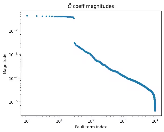
obs_tilde_isa = obs_tilde_isa[np.argsort(np.abs(obs_tilde_isa.coeffs))][::-1]
plt.xscale("log")
plt.yscale("log")
plt.title(r"$\tilde{O}$ coeff magnitudes")
plt.ylabel("Magnitude")
plt.xlabel("Pauli term index")
plt.plot(np.abs(obs_tilde_isa.coeffs), ".")

Output:

[<matplotlib.lines.Line2D at 0x124a07230>]

Transform the measurement bases to canonical form

Next, we will find a minimal set of bases to measure such that we can fully cover every Pauli term in the measured observable (many observables may be measured simultaneously if they commute qubit-wise). Since we are only measuring the terms in our original observable, which is the sum of all single-Z Paulis, a single basis is needed -- the all-Z basis.

In addition to finding a set of Pauli measurement bases, we need to map these Pauli terms to the canonical form expected by the Executor. For more information on canonical qubit ordering, visit the samplomatic docs.

meas_box = boxed_circuit.data[-1]
canonical_qubits = [
    idx
    for idx, qubit in enumerate(boxed_circuit.qubits)
    if qubit in meas_box.qubits
]
c_2_p = {
    c: p for c, p in enumerate(canonical_qubits)
}  # canonical -> physical
p_2_v = {p: v for v, p in enumerate(layout)}  # physical -> virtual
c_2_v = {c: p_2_v[p] for c, p in c_2_p.items()}  # canonical -> virtual
meas_bases, bases_reverser = get_measurement_bases(obs_tilde_virtual)
meas_bases_canonical = [
    np.array([base[c_2_v[c]] for c in range(num_qubits)], dtype=np.uint8)
    for base in meas_bases
]

Step 3: Execute quantum experiments

Specify how to sample in the QuantumProgram

We now set up the QuantumProgram, which serves as the central container for all circuits and sampling configurations that will be executed by the Executor. This object defines how randomized circuit instances are generated, batched, and executed to produce the measurement results used in PNA.

A QuantumProgram can contain multiple items, each consisting of a template circuit and a corresponding samplex object that defines how randomizations are applied. This abstraction allows the Executor to handle the entire workflow -- from randomized circuit generation to shot collection and aggregation -- as a single, modular program.

In this step, we create a QuantumProgram that runs our PNA experiment using the template circuit and samplex we constructed earlier. The configuration includes the following elements:

• template_circuit: The circuit containing all the gates necessary to implement all desired randomizations (from twirling randomizations, parameters, and so on).
• samplex: An object defining a probability distribution over all possible circuit randomizations from which to sample.
• samplex_arguments: Bindings necessary to fully define the samplex
  • basis_changes: Here is where we specify a set of bases to measure that will cover all of the Pauli terms in the measured observable.
  • noise_scales.ref: We set each noise layer's scale to 0.0 to prevent any additional noise from being injected into our samples.
  • pauli_lindblad_maps: Required if noise_scales are passed. This just maps noise layers to the associated noise model.
• shape: A shape tuple to extend the implicit shape defined by samplex_arguments. Non-trivial axes introduced by this extension enumerate randomizations.

# Control the # of shots during execution
shots_per_randomization_exec = 64
num_randomizations_exec = 6144

# Zero out the noise to prevent noise from being injected during execution.
# We only added InjectNoise annotations so PNA could associate the noise
# to layers in the circuit
samplex_inputs = {f"noise_scales.{ref}": 0.0 for ref in refs_to_noise_models}
samplex_inputs |= {"pauli_lindblad_maps": refs_to_noise_models}

# Specify the bases to measure. The samplex exposes one basis-change input per
# ChangeBasis-annotated box; here a single all-Z basis covers every term. We
# look up the basis-change interface name rather than hardcoding an index, since
# the name depends on the circuit's box structure.
bases_broadcastable = np.expand_dims(np.array(meas_bases_canonical), axis=1)
samplex_inputs |= {
    spec.name: bases_broadcastable
    for spec in samplex.inputs().get_specs(r"^basis_changes\.")
}

# Convert samplex_inputs into a dict to pass to QuantumProgram
samplex_arguments = (
    samplex.inputs().make_broadcastable().bind(**samplex_inputs)
)

# Instantiate the QuantumProgram with the specified parameters
program = QuantumProgram(shots=shots_per_randomization_exec)
program.append_samplex_item(
    circuit=template_circuit,
    samplex=samplex,
    samplex_arguments=samplex_arguments,
    shape=(num_randomizations_exec,),
)

Sample the circuit using the Executor

Now that we have defined our QuantumProgram, executing the experiment is straightforward. We simply instantiate the Executor object, provide it the backend, and run the program.

# Execute (sample) the circuit
executor = Executor(backend)
job_exec = executor.run(program)
exec_results = job_exec.result()

Step 4: Reconstruct and analyze results

To calculate an error-mitigated expectation value, we will:

• Calculate the TREX scaling factors based on the learned noise affecting the measurements,
• Generate a mask for keeping only post-selected samples, and
• Use the executor_expectation_values function from qiskit-addon-utils for combining all of the data into an error-mitigated expectation value.

# Computing the TREX factors
measurement_noise_map = noise_learner_result[2].to_pauli_lindblad_map()
trex_rescale_factors = trex_factors(measurement_noise_map, bases_reverser)

# Post-select the results
post_selector = PostSelector.from_circuit(
    circuit=template_circuit, coupling_map=backend.coupling_map
)

# Compute the ps mask for filtering results
mask = post_selector.compute_mask(exec_results[0], strategy="edge")

# Compute expvals using post selected results
results = executor_expectation_values(
    exec_results[0]["meas"],
    bases_reverser,
    meas_basis_axis=0,
    avg_axis=1,
    measurement_flips=exec_results[0]["measurement_flips.meas"],
    pauli_signs=exec_results[0].get("pauli_signs", None),
    postselect_mask=mask,
    rescale_factors=trex_rescale_factors,
)

Compare mitigation strategies: PNA, PNA+TREX, PNA+PS, PNA+PS+TREX

We will compute and visualize expectation values for several mitigation variants using the Executor results.

bases_reverser_unmit = {Pauli("Z" * num_qubits): [observable]}
args = [
    (bases_reverser_unmit, None, None),
    (bases_reverser, None, None),
    (bases_reverser, None, trex_rescale_factors),
    (bases_reverser, mask, None),
    (bases_reverser, mask, trex_rescale_factors),
]

evs = []
for reverser, postsel_mask, factors in args:
    # Compute expvals using post selected results
    res_ps = executor_expectation_values(
        exec_results[0]["meas"],
        reverser,
        meas_basis_axis=0,
        avg_axis=1,
        measurement_flips=exec_results[0]["measurement_flips.meas"],
        pauli_signs=exec_results[0].get("pauli_signs", None),
        postselect_mask=postsel_mask,
        rescale_factors=factors,
    )
    res_ps = np.array(res_ps)
    evs.append(res_ps[:, 0][0])

experiments = ["PNA", "PNA+TREX", "PNA+PS", "PNA+PS+TREX"]
colors = ["#d9d9d9", "#b0b0b0", "#7f7f7f", "#4c4c4c"]
plt.bar(experiments, evs[1:], color=colors)
plt.axhline(y=1, color="green", linestyle="--", linewidth=2, label="Ideal")
plt.axhline(
    y=evs[0], color="red", linestyle="--", linewidth=2, label="Unmitigated"
)
plt.ylabel("Expectation value", fontsize=14)

plt.title(
    r"30q Mirrored Ising, 10 Trotter steps, $\theta_{rx}=\frac{\pi}{8}$",
    fontsize=14,
)
plt.legend(loc="upper left", bbox_to_anchor=(1.05, 1), borderaxespad=0.0)
plt.xticks(rotation=45)
plt.tight_layout()
plt.show()

Output:

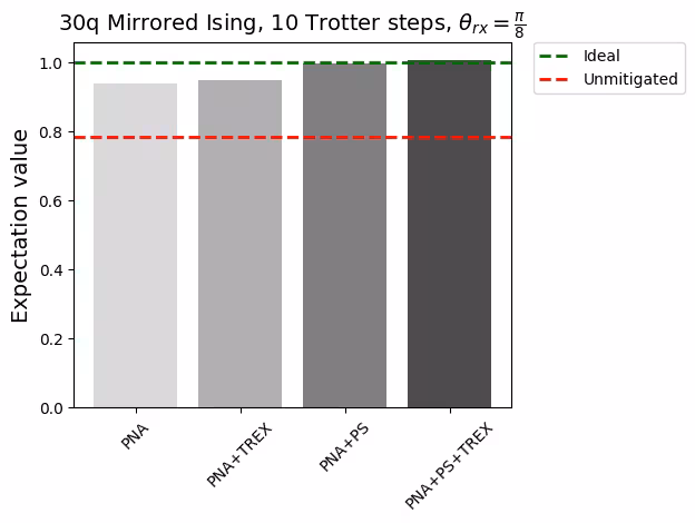
The results demonstrate the cumulative benefits of combining different error-mitigation techniques. The plain PNA approach already restores the expectation value close to the ideal benchmark, indicating that propagating inverse noise channels into the observable effectively compensates for two-qubit gate errors.

• Adding TREX reweighting (PNA+TREX) slightly improves the estimate by correcting for sampling imbalance in the randomized circuits.
• Post-selection (PNA+PS) provides a more noticeable boost by filtering out inconsistent measurement outcomes that likely result from residual errors.
• Finally, combining both (PNA+PS+TREX) yields the most accurate result, nearly matching the ideal value, showing how these mitigation strategies reinforce each other.

Overall, the comparison highlights that PNA serves as a robust foundation for noise-aware expectation value estimation, while TREX and post-selection offer complementary refinements for further accuracy gains.

Next steps

If you found this work interesting, you might be interested in the following material: