CHSH inequality
Usage estimate: Two minutes on a Heron r3 processor (NOTE: This is an estimate only. Your runtime might vary.)
Learning outcomes
After completing this tutorial, you can expect to understand the following information:
- How to construct a parameterized Bell-state CHSH circuit and measure the four expectation values that make up the CHSH witnesses.
- How to compute expectation values of multiple observables on a parameter sweep in a single call to the
EstimatorV2primitive. - How to validate a quantum workflow on a noisy local simulator with
AerSimulator.from_backendbefore submitting to hardware. - How to scale a CHSH experiment into a device-wide entanglement benchmark by running many independent Bell pairs in parallel on IBM Quantum® hardware.
Prerequisites
It is recommended that you familiarize yourself with these topics:
- Entanglement in action, a course lesson on Bell states and the CHSH game.
SparsePauliOpand the Qiskit primitives introduction.
Background
In this tutorial, you will run an experiment on a quantum computer to demonstrate the violation of the CHSH inequality with the Estimator primitive.
The CHSH inequality, named after Clauser, Horne, Shimony, and Holt, is used to experimentally test Bell's theorem (1969). The theorem asserts that local hidden-variable theories cannot account for some consequences of entanglement in quantum mechanics. Demonstrating a violation of the CHSH inequality shows that quantum mechanics is incompatible with local hidden-variable theories, an experiment that is foundational to our understanding of quantum mechanics.
The 2022 Nobel Prize for Physics was awarded to Alain Aspect, John Clauser, and Anton Zeilinger in part for their pioneering work in quantum information science, and in particular, for their experiments with entangled photons demonstrating violation of Bell's inequalities.
For this experiment, we will create an entangled pair on which we measure each qubit in two different bases. We will label the bases for the first qubit and and the bases for the second qubit and . This allows us to compute the CHSH quantity :
Each observable is either or . Clearly, one of the terms must be , and the other must be . Therefore, . The average value of must satisfy the inequality:
Expanding in terms of , , , and gives:
You can define another CHSH quantity :
which leads to another inequality:
If quantum mechanics could be described by local hidden-variable theories, these inequalities would always hold. As demonstrated in this tutorial, they can be violated on a quantum computer, so quantum mechanics is not compatible with local hidden-variable theories.
We create the entangled pair by preparing the Bell state . Using the Estimator primitive, we obtain the expectation values , and directly, without reconstructing them from raw counts. We measure the second qubit in the and bases. The first qubit is measured in orthogonal bases as well, but with a rotation angle that we sweep between and . The Estimator primitive evaluates this parameter sweep in a single primitive unified bloc (PUB).
Requirements
Before starting this tutorial, be sure you have the following installed:
- Qiskit SDK v2.0 or later, with visualization support
- Qiskit Runtime v0.40 or later (
pip install qiskit-ibm-runtime) - Qiskit Aer v0.17 or later (
pip install qiskit-aer)
Setup
# General
import numpy as np

# Qiskit imports
from qiskit import QuantumCircuit
from qiskit.circuit import Parameter
from qiskit.quantum_info import SparsePauliOp
from qiskit.transpiler.preset_passmanagers import generate_preset_pass_manager

# Qiskit Runtime imports
from qiskit_ibm_runtime import QiskitRuntimeService
from qiskit_ibm_runtime import EstimatorV2 as Estimator

# Qiskit Aer for local noisy simulation
from qiskit_aer import AerSimulator

# Plotting routines
import matplotlib.pyplot as plt
import matplotlib.ticker as tck
# Select an IBM Quantum backend.
service = QiskitRuntimeService()
backend = service.least_busy(
min_num_qubits=127, operational=True, simulator=False
)
backend.nameOutput:
'ibm_pittsburgh'
Small-scale simulator example
Before submitting a hardware job, we validate the entire workflow on a local noisy simulator. We use AerSimulator.from_backend(backend) to build a simulator that inherits the noise model and coupling map of the backend you selected, so the simulator response is qualitatively similar to what we expect from hardware.
Step 1: Map classical inputs to a quantum problem
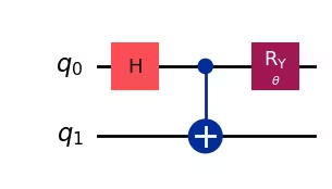
We write the CHSH circuit with a single parameter , which sweeps the measurement basis of the first qubit. The Estimator primitive simplifies the analysis: it returns expectation values of observables directly, and it can evaluate a parameterized circuit at many parameter values in a single call.
theta = Parameter(r"$\theta$")

chsh_circuit = QuantumCircuit(2)
chsh_circuit.h(0)
chsh_circuit.cx(0, 1)
chsh_circuit.ry(theta, 0)
chsh_circuit.draw(output="mpl", idle_wires=False, style="iqp")
Output:
Next, we create a list of 21 phase values from to at which to evaluate the parameterized circuit (, , , ..., , ).
number_of_phases = 21
phases = np.linspace(0, 2 * np.pi, number_of_phases)
# Phases need to be expressed as a list of lists for the Estimator PUB
individual_phases = [[ph] for ph in phases]
Finally we define the observables. The first qubit is measured along axes rotated by ; the second qubit is measured in and . With those choices, the four CHSH correlators map to the Pauli operators , , , and :
# <S_1> = <ZZ> - <ZX> + <XZ> + <XX>
observable1 = SparsePauliOp.from_list(
    [("ZZ", 1), ("ZX", -1), ("XZ", 1), ("XX", 1)]
)

# <S_2> = <ZZ> + <ZX> - <XZ> + <XX>
observable2 = SparsePauliOp.from_list(
    [("ZZ", 1), ("ZX", 1), ("XZ", -1), ("XX", 1)]
)
Step 2: Optimize problem for quantum hardware execution
V2 primitives only accept circuits and observables that conform to the instructions and connectivity supported by the target system (instruction set architecture, or ISA, circuits and observables). We build the AerSimulator from the backend and transpile against the simulator's target so the same pass manager is exercised end-to-end.
# Build a noisy simulator from the ibm_pittsburgh backend
aer_sim = AerSimulator.from_backend(backend)

pm = generate_preset_pass_manager(target=aer_sim.target, optimization_level=3)
chsh_isa_circuit = pm.run(chsh_circuit)
chsh_isa_circuit.draw(output="mpl", idle_wires=False, style="iqp")
Output:
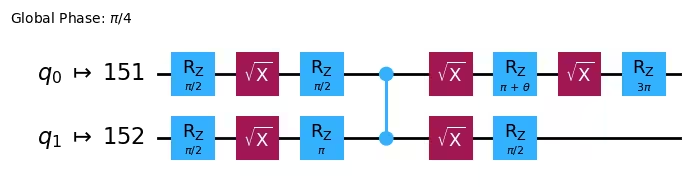
We also transform the observables to match the transpiled circuit's qubit layout using SparsePauliOp.apply_layout.
isa_observable1 = observable1.apply_layout(layout=chsh_isa_circuit.layout)
isa_observable2 = observable2.apply_layout(layout=chsh_isa_circuit.layout)
Step 3: Execute using Qiskit primitives
Run the parameter sweep with EstimatorV2 in aer_sim mode. The Estimator run() method takes an iterable of PUBs. Each PUB has the format (circuit, observables, parameter_values, precision). We pass both observables together so they share the same parameter sweep.
# Use the AerSimulator-backed Estimator to validate the workflow locally
estimator_sim = Estimator(mode=aer_sim)

pub = (
    chsh_isa_circuit,  # ISA circuit
    [[isa_observable1], [isa_observable2]],  # ISA observables
    individual_phases,  # Parameter values
)

sim_result = estimator_sim.run(pubs=[pub]).result()
Step 4: Post-process and return result in desired classical format
The Estimator returns expectation values for both observables. We plot them against together with the classical bound () and the Tsirelson bound (). The shaded grey regions mark the gap between the two. Points that lie inside these bands violate the CHSH inequality.
chsh1_sim = sim_result[0].data.evs[0]
chsh2_sim = sim_result[0].data.evs[1]


def plot_chsh(phases, chsh1, chsh2, title):
    fig, ax = plt.subplots(figsize=(10, 6))

    ax.plot(
        phases / np.pi, chsh1, "o-", label=r"$\langle S_1 \rangle$", zorder=3
    )
    ax.plot(
        phases / np.pi, chsh2, "o-", label=r"$\langle S_2 \rangle$", zorder=3
    )

    # classical bound +-2
    ax.axhline(y=2, color="0.9", linestyle="--")
    ax.axhline(y=-2, color="0.9", linestyle="--")

    # quantum bound, +-2*sqrt(2)
    ax.axhline(y=np.sqrt(2) * 2, color="0.9", linestyle="-.")
    ax.axhline(y=-np.sqrt(2) * 2, color="0.9", linestyle="-.")
    ax.fill_between(phases / np.pi, 2, 2 * np.sqrt(2), color="0.6", alpha=0.7)
    ax.fill_between(
        phases / np.pi, -2, -2 * np.sqrt(2), color="0.6", alpha=0.7
    )

    ax.xaxis.set_major_formatter(tck.FormatStrFormatter("%g $\\pi$"))
    ax.xaxis.set_major_locator(tck.MultipleLocator(base=0.5))

    ax.set_xlabel(r"$\theta$")
    ax.set_ylabel("CHSH witness")
    ax.set_title(title)
    ax.legend()
    plt.show()


plot_chsh(
    phases,
    chsh1_sim,
    chsh2_sim,
    "CHSH witnesses from AerSimulator (ibm_pittsburgh noise model)",
)
Output:
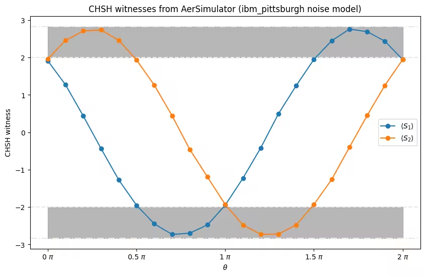
The simulator's CHSH witnesses already exceed the classical bound of at several values of , even with the backend's noise model. The peaks fall just short of the Tsirelson bound because of simulated device noise. With the workflow validated, we move on to actual hardware.
Large-scale hardware example
A CHSH test is intrinsically a two-qubit experiment, so it does not scale by making one circuit bigger. Instead, it scales by running many tests in parallel. Here we tile the backend with as many disjoint Bell pairs as its connectivity allows (a matching of the coupling map) and run an independent CHSH sub-circuit on every pair, all in a single job.
This turns CHSH into a device-wide benchmark of entanglement quality: rather than a single hand-picked pair, we test entanglement across a large fraction of the chip at once, under realistic conditions where every pair contends with its neighbors' crosstalk and parallel-gate errors. Violating the inequality on every pair simultaneously certifies that genuine entanglement is available everywhere on the device.
# -------------------------Step 1: Map classical inputs to a quantum problem-------------------------
# A CHSH test is bipartite, so we scale up by running one independent CHSH
# experiment on every disjoint Bell pair the device can host. A greedy
# matching of the coupling map gives a set of edges that share no qubits.
num_qubits = backend.num_qubits
used = set()
pairs = []
for qa, qb in backend.coupling_map.get_edges():
    if qa not in used and qb not in used:
        pairs.append((qa, qb))
        used.update((qa, qb))
num_pairs = len(pairs)
print(
    f"Tiling {backend.name} with {num_pairs} parallel Bell pairs "
    f"({2 * num_pairs} of {num_qubits} qubits)"
)

# One parameterized CHSH sub-circuit per pair, all sharing the angle theta
theta = Parameter(r"$\theta$")
chsh_circuit = QuantumCircuit(num_qubits)
for qa, qb in pairs:
    chsh_circuit.h(qa)
    chsh_circuit.cx(qa, qb)
    chsh_circuit.ry(theta, qa)

# Embed the two CHSH observables onto each pair's qubits (identity elsewhere)
obs1 = SparsePauliOp.from_list([("ZZ", 1), ("ZX", -1), ("XZ", 1), ("XX", 1)])
obs2 = SparsePauliOp.from_list([("ZZ", 1), ("ZX", 1), ("XZ", -1), ("XX", 1)])
observables = []
for qa, qb in pairs:
    observables.append([obs1.apply_layout([qa, qb], num_qubits)])
    observables.append([obs2.apply_layout([qa, qb], num_qubits)])

number_of_phases = 21
phases = np.linspace(0, 2 * np.pi, number_of_phases)
individual_phases = [[ph] for ph in phases]

# -------------------------Step 2: Optimize problem for quantum hardware execution-------------------------
pm = generate_preset_pass_manager(target=backend.target, optimization_level=3)
chsh_isa_circuit = pm.run(chsh_circuit)
isa_observables = [
    [o[0].apply_layout(chsh_isa_circuit.layout)] for o in observables
]

# -------------------------Step 3: Execute using Qiskit primitives-------------------------
estimator_hw = Estimator(mode=backend)
estimator_hw.options.environment.job_tags = ["TUT_CI"]

pub = (chsh_isa_circuit, isa_observables, individual_phases)
job = estimator_hw.run(pubs=[pub])
print(f"Job ID: {job.job_id()}")
hw_result = job.result()

# -------------------------Step 4: Post-process and return result in desired classical format-------------------------
# evs has shape (2 * num_pairs, number_of_phases); rows alternate S1, S2
evs = np.asarray(hw_result[0].data.evs)
chsh1_all = evs[0::2]
chsh2_all = evs[1::2]

# A pair "violates" CHSH if its strongest witness exceeds the classical bound
peak = np.maximum(
    np.abs(chsh1_all).max(axis=1), np.abs(chsh2_all).max(axis=1)
)
n_violate = int(np.sum(peak > 2))
print(
    f"{n_violate}/{num_pairs} Bell pairs violated the CHSH inequality "
    f"(mean peak witness {peak.mean():.2f}, classical bound 2)"
)

fig, ax = plt.subplots(figsize=(10, 6))

# Faint individual per-pair curves
for row in chsh1_all:
    ax.plot(phases / np.pi, row, color="#1f77b4", alpha=0.2, lw=1)
for row in chsh2_all:
    ax.plot(phases / np.pi, row, color="#ff7f0e", alpha=0.2, lw=1)

# Bold mean curves across all pairs
ax.plot(
    phases / np.pi,
    chsh1_all.mean(axis=0),
    color="#1f77b4",
    lw=2.5,
    label=r"$\langle S_1 \rangle$ (mean)",
)
ax.plot(
    phases / np.pi,
    chsh2_all.mean(axis=0),
    color="#ff7f0e",
    lw=2.5,
    label=r"$\langle S_2 \rangle$ (mean)",
)

# classical bound +-2 and Tsirelson bound +-2*sqrt(2)
ax.axhline(y=2, color="0.9", linestyle="--")
ax.axhline(y=-2, color="0.9", linestyle="--")
ax.axhline(y=np.sqrt(2) * 2, color="0.9", linestyle="-.")
ax.axhline(y=-np.sqrt(2) * 2, color="0.9", linestyle="-.")
ax.fill_between(phases / np.pi, 2, 2 * np.sqrt(2), color="0.6", alpha=0.7)
ax.fill_between(phases / np.pi, -2, -2 * np.sqrt(2), color="0.6", alpha=0.7)

ax.xaxis.set_major_formatter(tck.FormatStrFormatter("%g $\\pi$"))
ax.xaxis.set_major_locator(tck.MultipleLocator(base=0.5))
ax.set_xlabel(r"$\theta$")
ax.set_ylabel("CHSH witness")
ax.set_title(
    f"CHSH witnesses for {num_pairs} parallel Bell pairs on {backend.name}"
)
ax.legend()
plt.show()
Output:
Tiling ibm_pittsburgh with 64 parallel Bell pairs (128 of 156 qubits)
Job ID: d86efd5g7okc73el0rp0
63/64 Bell pairs violated the CHSH inequality (mean peak witness 2.75, classical bound 2)
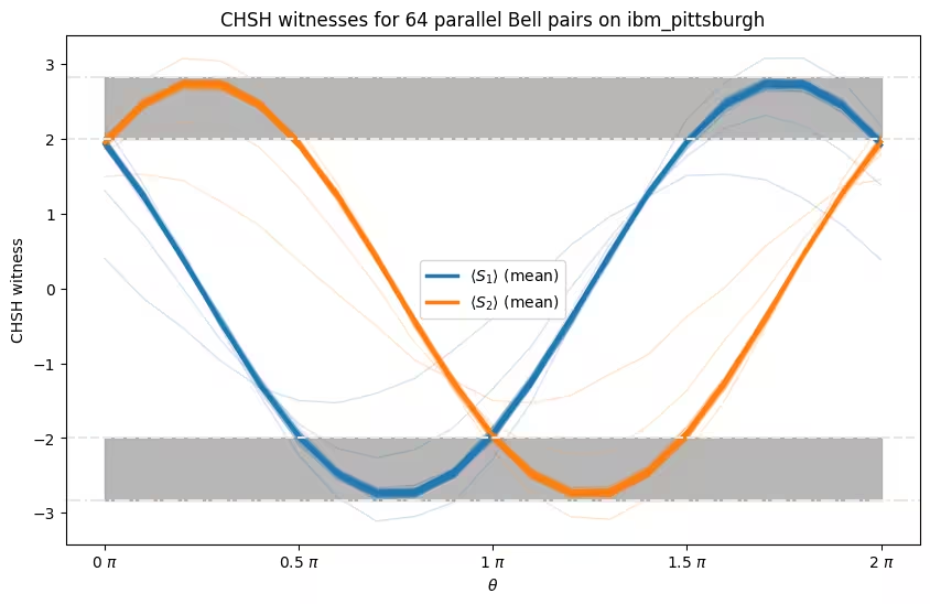
The faint curves are the individual Bell pairs and the bold curves are their mean across the device. Every pair traces the same sinusoid predicted by quantum mechanics, and the spread between the faint curves reflects the variation in noise from pair to pair. Wherever a curve enters the grey bands, it has crossed the classical bound of , and the printed summary confirms that essentially every pair violates the CHSH inequality at the same time.
The peaks fall short of the Tsirelson bound because of device noise, but the conclusion is unambiguous: the backend sustains genuine entanglement across the whole chip simultaneously, not just on a single hand-picked pair. This is the sense in which the CHSH experiment "scales": not as one larger circuit, but as a parallel benchmark that certifies entanglement everywhere at once.
Next steps
If you found this work interesting, you might be interested in the following material:
- Entanglement in action: a course lesson by John Watrous on Bell states and the CHSH game.
- Get started with the Estimator primitive: a guide on PUBs and parameter sweeps.
- Real-time benchmarking for qubit selection: another way to characterize qubit and entanglement quality across a device.
SparsePauliOpAPI reference.