Grover's algorithm

Usage estimate: under one minute on Eagle r3 processor (NOTE: This is an estimate only. Your runtime might vary.)

Learning outcomes

After completing this tutorial, you can expect to understand the following information:

• How to construct Grover oracles that mark one or more computational basis states
• How to use the grover_operator() function from the Qiskit circuit library
• How to determine the optimal number of Grover iterations for a given problem
• How to execute Grover's algorithm using the Qiskit Runtime Sampler primitive

Prerequisites

It is recommended that you familiarize yourself with these topics:

• Fundamentals of quantum algorithms: Grover's algorithm
• Basics of quantum information

Background

Amplitude amplification is a general purpose quantum algorithm, or subroutine, that can be used to obtain a quadratic speedup over a handful of classical algorithms. Grover's algorithm was the first to demonstrate this speedup on unstructured search problems. Formulating a Grover's search problem requires an oracle function that marks one or more computational basis states as the states we are interested in finding, and an amplification circuit that increases the amplitude of marked states, consequently suppressing the remaining states.

Here, we demonstrate how to construct Grover oracles and use the grover_operator() from the Qiskit circuit library to easily set up a Grover's search instance. The runtime Sampler primitive allows seamless execution of Grover circuits.

Requirements

Before starting this tutorial, be sure you have the following installed:

• Qiskit SDK v2.0 or later, with visualization support
• Qiskit Runtime v0.22 or later (pip install qiskit-ibm-runtime)

Setup

# Built-in modules
import math

# Imports from Qiskit
from qiskit import QuantumCircuit
from qiskit.circuit.library import grover_operator, MCMTGate, ZGate
from qiskit.visualization import plot_distribution
from qiskit.transpiler.preset_passmanagers import generate_preset_pass_manager

# Imports from Qiskit Runtime
from qiskit_ibm_runtime import QiskitRuntimeService
from qiskit_ibm_runtime import SamplerV2 as Sampler


def grover_oracle(marked_states):
    """Build a Grover oracle for multiple marked states

    Here we assume all input marked states have the same number of bits

    Parameters:
        marked_states (str or list): Marked states of oracle

    Returns:
        QuantumCircuit: Quantum circuit representing Grover oracle
    """
    if not isinstance(marked_states, list):
        marked_states = [marked_states]
    # Compute the number of qubits in circuit
    num_qubits = len(marked_states[0])

    qc = QuantumCircuit(num_qubits)
    # Mark each target state in the input list
    for target in marked_states:
        # Flip target bit-string to match Qiskit bit-ordering
        rev_target = target[::-1]
        # Find the indices of all the '0' elements in bit-string
        zero_inds = [
            ind
            for ind in range(num_qubits)
            if rev_target.startswith("0", ind)
        ]
        # Add a multi-controlled Z-gate with pre- and post-applied X-gates (open-controls)
        # where the target bit-string has a '0' entry
        if zero_inds:
            qc.x(zero_inds)
        qc.compose(MCMTGate(ZGate(), num_qubits - 1, 1), inplace=True)
        if zero_inds:
            qc.x(zero_inds)
    return qc

Small-scale simulator example

In this section, we walk through each step of Grover's algorithm at a small scale using a local simulator, before running the same problem on real quantum hardware.

Step 1: Map classical inputs to a quantum problem

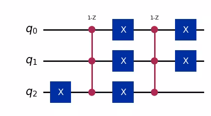
Grover's algorithm requires an oracle that specifies one or more marked computational basis states, where "marked" means a state with a phase of -1. A controlled-Z gate, or its multi-controlled generalization over $N$ qubits, marks the $2^{N}-1$ state ('1'*$N$ bit-string). Marking basis states with one or more '0' in the binary representation requires applying X-gates on the corresponding qubits before and after the controlled-Z gate; equivalent to having an open-control on that qubit. In the following code, we define an oracle that does just that, marking one or more input basis states defined through their bit-string representation. The MCMT gate is used to implement the multi-controlled Z-gate.

Specific Grover's instance

Now that we have the oracle function, we can define a specific instance of Grover search. In this example we will mark two computational states out of the eight available in a three-qubit computational space:

marked_states = ["011", "100"]

oracle = grover_oracle(marked_states)
oracle.draw(output="mpl", style="iqp")

Output:

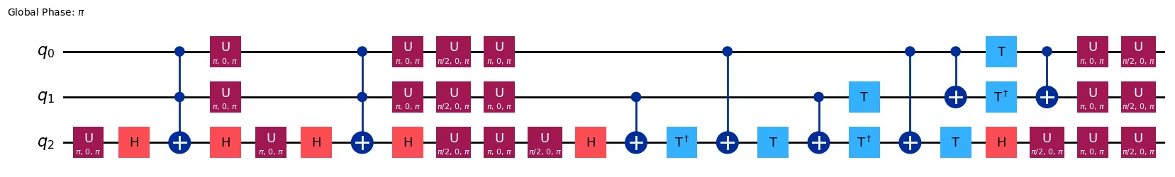
Grover operator

The built-in Qiskit grover_operator() takes an oracle circuit and returns a circuit that is composed of the oracle circuit itself and a circuit that amplifies the states marked by the oracle. Here, we use the decompose() method the circuit to see the gates within the operator:

grover_op = grover_operator(oracle)
grover_op.decompose().draw(output="mpl", style="iqp")

Output:

Repeated applications of this grover_op circuit amplify the marked states, making them the most probable bit-strings in the output distribution from the circuit. There is an optimal number of such applications that is determined by the ratio of marked states to total number of possible computational states:

optimal_num_iterations = math.floor(
    math.pi
    / (4 * math.asin(math.sqrt(len(marked_states) / 2**grover_op.num_qubits)))
)

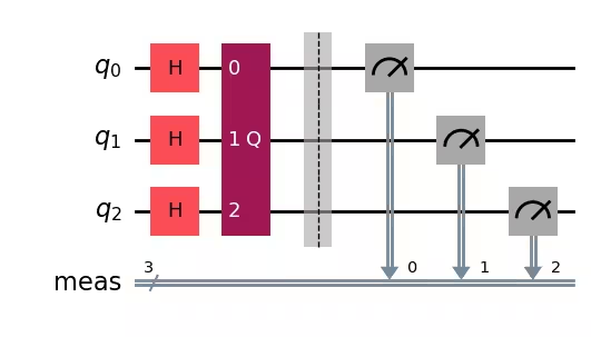
Full Grover circuit

A complete Grover experiment starts with a Hadamard gate on each qubit; creating an even superposition of all computational basis states, followed the Grover operator (grover_op) repeated the optimal number of times. Here we make use of the QuantumCircuit.power(INT) method to repeatedly apply the Grover operator.

qc = QuantumCircuit(grover_op.num_qubits)
# Create even superposition of all basis states
qc.h(range(grover_op.num_qubits))
# Apply Grover operator the optimal number of times
qc.compose(grover_op.power(optimal_num_iterations), inplace=True)
# Measure all qubits
qc.measure_all()
qc.draw(output="mpl", style="iqp")

Output:

Step 2: Optimize problem for quantum hardware execution

For the small-scale simulation, we transpile the circuit without targeting specific hardware.

pm = generate_preset_pass_manager(optimization_level=3)
circuit_isa = pm.run(qc)
circuit_isa.draw(output="mpl", idle_wires=False, style="iqp")

Output:

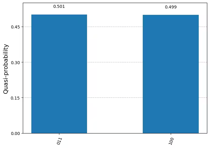
Step 3: Execute using Qiskit primitives

Amplitude amplification is a sampling problem that is suitable for execution with the SamplerV2 runtime primitive. Here we use the StatevectorSampler from qiskit.primitives for local simulation.

from qiskit.primitives import StatevectorSampler

sampler = StatevectorSampler()
result = sampler.run([circuit_isa], shots=10_000).result()
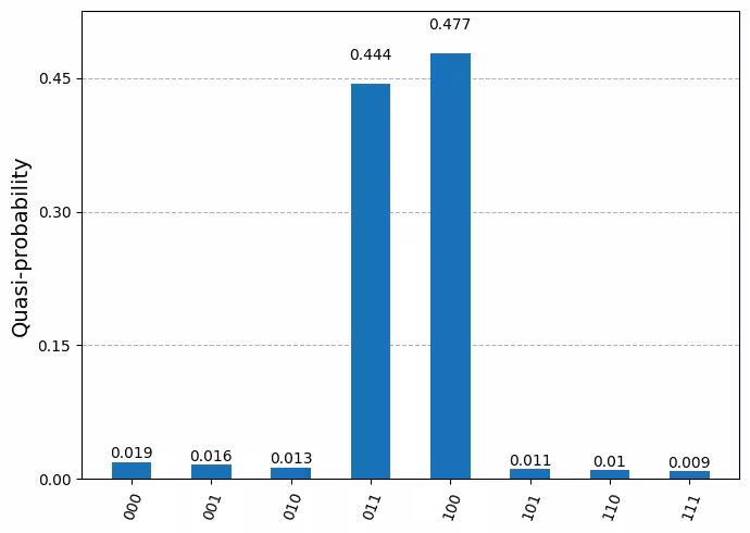
dist = result[0].data.meas.get_counts()

Step 4: Post-process and return result in desired classical format

plot_distribution(dist)

Output:

Hardware example

Steps 1-4 compress into single code block

Grover's algorithm is fundamentally a fault-tolerant algorithm — the multi-controlled Z gates at the heart of the oracle and diffusion operator lead to two-qubit gate depths that grow very rapidly with the number of qubits (as we will show in the next section). This means the algorithm does not scale well on today's noisy hardware. For this reason, we demonstrate the hardware execution at the same small scale as the simulator example above, rather than attempting a larger problem size.

# -------------------------Step 1-------------------------
marked_states = ["011", "100"]

oracle = grover_oracle(marked_states)
grover_op = grover_operator(oracle)

optimal_num_iterations = math.floor(
    math.pi
    / (4 * math.asin(math.sqrt(len(marked_states) / 2**grover_op.num_qubits)))
)

qc = QuantumCircuit(grover_op.num_qubits)
qc.h(range(grover_op.num_qubits))
qc.compose(grover_op.power(optimal_num_iterations), inplace=True)
qc.measure_all()

# -------------------------Step 2-------------------------
service = QiskitRuntimeService()
backend = service.least_busy(
    operational=True, simulator=False, min_num_qubits=127
)

target = backend.target
pm = generate_preset_pass_manager(target=target, optimization_level=3)
circuit_isa = pm.run(qc)

# -------------------------Step 3-------------------------
sampler = Sampler(mode=backend)
sampler.options.default_shots = 10_000
sampler.options.environment.job_tags = ["TUT-GA"]
result = sampler.run([circuit_isa]).result()
dist = result[0].data.meas.get_counts()

# -------------------------Step 4-------------------------
plot_distribution(dist)

Output:

Discussion: Two-qubit gate depth scaling

A key reason Grover's algorithm is considered a fault-tolerant algorithm is the rapid growth of the circuit's two-qubit gate depth as the number of qubits increases. The multi-controlled Z gate at the core of both the oracle and the diffusion operator decomposes into a number of two-qubit gates that grows exponentially with the number of control qubits. Combined with the fact that the optimal number of Grover iterations itself grows as $O(\sqrt{2^n})$, the overall two-qubit depth quickly becomes impractical for noisy hardware.

Below, we construct Grover circuits for increasing qubit counts, transpile them, and plot the resulting two-qubit gate depth to illustrate this scaling.

import matplotlib.pyplot as plt

num_qubits_list = list(range(3, 10))
two_q_depths = []
backend = service.least_busy(
    operational=True, simulator=False, min_num_qubits=127
)
for n in num_qubits_list:
    # Mark a single state for simplicity
    marked = ["1" * n]
    oracle_n = grover_oracle(marked)
    grover_op_n = grover_operator(oracle_n)

    # Optimal number of iterations
    num_iters = math.floor(
        math.pi / (4 * math.asin(math.sqrt(len(marked) / 2**n)))
    )

    # Build the full Grover circuit
    qc_n = QuantumCircuit(n)
    qc_n.h(range(n))
    qc_n.compose(grover_op_n.power(num_iters), inplace=True)
    qc_n.measure_all()

    # Transpile to a basis gate set and count 2Q depth
    pm_n = generate_preset_pass_manager(backend=backend, optimization_level=3)
    qc_transpiled = pm_n.run(qc_n)

    # Compute depth restricted to 2-qubit operations
    depth_2q = qc_transpiled.depth(lambda x: x.operation.num_qubits == 2)

    two_q_depths.append(depth_2q)
    print(f"n={n}: optimal_iters={num_iters}, 2Q depth={depth_2q}")

# Plot
fig, ax = plt.subplots(figsize=(8, 5))
ax.plot(
    num_qubits_list,
    two_q_depths,
    "o-",
    linewidth=2,
    markersize=8,
    color="#6929C4",
)
ax.set_xlabel("Number of qubits", fontsize=13)
ax.set_ylabel("Two-qubit gate depth", fontsize=13)
ax.set_title("Grover's algorithm: 2Q depth scaling", fontsize=14)
ax.set_yscale("log")
ax.grid(True, alpha=0.3)
ax.set_xticks(num_qubits_list)
plt.tight_layout()
plt.show()

Output:

n=3: optimal_iters=2, 2Q depth=39
n=4: optimal_iters=3, 2Q depth=111
n=5: optimal_iters=4, 2Q depth=466
n=6: optimal_iters=6, 2Q depth=1646
n=7: optimal_iters=8, 2Q depth=3550
n=8: optimal_iters=12, 2Q depth=7989
n=9: optimal_iters=17, 2Q depth=14824

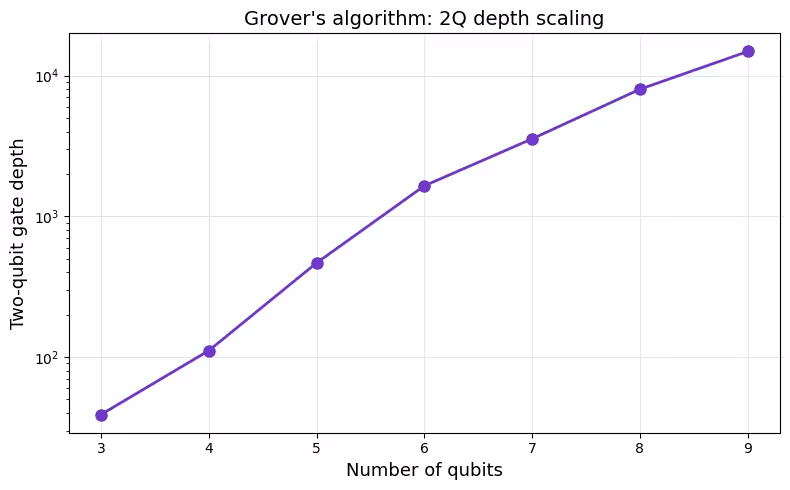
As the plot shows, the two-qubit gate depth grows extremely rapidly with the number of qubits — roughly exponentially. This makes Grover's algorithm impractical on current noisy quantum hardware beyond very small problem sizes. The algorithm remains an important target for future fault-tolerant quantum computers, where error correction will allow deep circuits to be executed reliably.

Next steps

If you found this work interesting, you might be interested in the following material: