Sample-based Krylov quantum diagonalization of a fermionic lattice model

Usage estimate: Nine seconds on a Heron r2 processor (NOTE: This is an estimate only. Your runtime might vary.)

Learning outcomes

After going through this tutorial, users should understand:

How to use the SQD Qiskit addon to approximate the ground state energy of a lattice model using bitstrings sampled from a quantum processing unit (QPU).
How to use ffsim to construct time evolution circuits for fermionic simulation.
How to combine samples from multiple circuits for post-processing with the sample-based Krylov diagonalization (SKQD) algorithm.

Prerequisites

We suggest that users are familiar with the following topics before going through this tutorial:

Background

This tutorial shows how to use sample-based quantum diagonalization (SQD) to estimate the ground state energy of a fermionic lattice model. Specifically, we study the one-dimensional single-impurity Anderson model (SIAM), which is used to describe magnetic impurities embedded in metals.

This tutorial follows a similar workflow to the related tutorial Sample-based quantum diagonalization of a chemistry Hamiltonian. However, a key difference lies in how the quantum circuits are built. The other tutorial uses a heuristic variational ansatz, which is appealing for chemistry Hamiltonians with potentially millions of interaction terms. On the other hand, this tutorial uses circuits that approximate time evolution by the Hamiltonian. Such circuits can be deep, which makes this approach better for applications to lattice models. The state vectors prepared by these circuits form the basis for a Krylov subspace, and as a result, the algorithm provably and efficiently converges to the ground state, under suitable assumptions.

The approach used in this tutorial can be viewed as a combination of the techniques used in SQD and Krylov quantum diagonalization (KQD). The combined approach is sometimes referred to as sample-based Krylov quantum diagonalization (SQKD). See Krylov quantum diagonalization of lattice Hamiltonians for a tutorial on the KQD method.

This tutorial is based on the work "Quantum-Centric Algorithm for Sample-Based Krylov Diagonalization", which can be referred to for more details.

Single-impurity Anderson model (SIAM)

The one-dimensional SIAM Hamiltonian is a sum of three terms:

H = H_{\textrm{imp}}+ H_\textrm{bath} + H_\textrm{hyb},

where

\begin{align*} H_\textrm{imp} &= \varepsilon \left( \hat{n}_{d\uparrow} + \hat{n}_{d\downarrow} \right) + U \hat{n}_{d\uparrow}\hat{n}_{d\downarrow}, \\ H_\textrm{bath} &= -t \sum_{\substack{\mathbf{j} = 0\\ \sigma\in \{\uparrow, \downarrow\}}}^{L-1} \left(\hat{c}^\dagger_{\mathbf{j}, \sigma}\hat{c}_{\mathbf{j}+1, \sigma} + \hat{c}^\dagger_{\mathbf{j}+1, \sigma}\hat{c}_{\mathbf{j}, \sigma} \right), \\ H_\textrm{hyb} &= V\sum_{\sigma \in \{\uparrow, \downarrow \}} \left(\hat{d}^\dagger_\sigma \hat{c}_{0, \sigma} + \hat{c}^\dagger_{0, \sigma} \hat{d}_{\sigma} \right). \end{align*}

Here, $c^\dagger_{\mathbf{j},\sigma}/c_{\mathbf{j},\sigma}$ are the fermionic creation/annihilation operators for the $\mathbf{j}^{\textrm{th}}$ bath site with spin $\sigma$ , $\hat{d}^\dagger_{\sigma}/\hat{d}_{\sigma}$ are creation/annihilation operators for the impurity mode, and $\hat{n}_{d\sigma} = \hat{d}^\dagger_{\sigma} \hat{d}_{\sigma}$ . $t$ , $U$ , and $V$ are real numbers describing the hopping, on-site, hybridization interactions, and $\varepsilon$ is a real number specifying the chemical potential.

Note that the Hamiltonian is a specific instance of the generic interaction-electron Hamiltonian,

\begin{align*} H &= \sum_{\substack{p, q \\ \sigma}} h_{pq} \hat{a}^\dagger_{p\sigma} \hat{a}_{q\sigma} + \sum_{\substack{p, q, r, s \\ \sigma \tau}} \frac{h_{pqrs}}{2} \hat{a}^\dagger_{p\sigma} \hat{a}^\dagger_{q\tau} \hat{a}_{s\tau} \hat{a}_{r\sigma} \\ &= H_1 + H_2, \end{align*}

where $H_1$ consists of one-body terms, which are quadratic in the fermionic creation and annihilation operators, and $H_2$ consists of two-body terms, which are quartic. For the SIAM,

H_2 = U \hat{n}_{d\uparrow}\hat{n}_{d\downarrow}

and $H_1$ contains the rest of the terms in the Hamiltonian. In order to represent the Hamiltonian programmatically, we store the matrix $h_{pq}$ and the tensor $h_{pqrs}$ .

Position and momentum bases

Due to the approximate translational symmetry in $H_\textrm{bath}$ , we don't expect the ground state to be sparse in the position basis (the orbital basis in which the Hamiltonian is specified above). The performance of SQD is guaranteed only if the ground state is sparse, that is, it has significant weight on only a small number of computational basis states. To improve the sparsity of the ground state, we perform the simulation in the orbital basis in which $H_\textrm{bath}$ is diagonal. We call this basis the momentum basis. Because $H_\textrm{bath}$ is a quadratic fermionic Hamiltonian, it can be efficiently diagonalized by an orbital rotation.

Approximate time evolution by the Hamiltonian

To approximate time evolution by the Hamiltonian, we use a second order Trotter-Suzuki decomposition,

e^{-i \Delta t H} \approx e^{-i\frac{\Delta t}{2} H_2} e^{-i\Delta t H_1} e^{-i\frac{\Delta t}{2} H_2}.

Under the Jordan-Wigner transformation, time evolution by $H_2$ amounts to a single CPhase gate between the spin-up and spin-down orbitals at the impurity site. Because $H_1$ is a quadratic fermionic Hamiltonian, time evolution by $H_1$ amounts to an orbital rotation.

The Krylov basis states $\{ |\psi_k\rangle \}_{k=0}^{D-1}$ , where $D$ is the dimension of the Krylov subspace, are formed by repeated application of a single Trotter step, so

|\psi_k\rangle \approx \left[e^{-i\frac{\Delta t}{2} H_2} e^{-i\Delta t H_1} e^{-i\frac{\Delta t}{2} H_2} \right]^k\ket{\psi_0}.

In the following SQD-based workflow, we will sample from this set of circuits and post-process the combined set of bitstrings with SQD. This approach contrasts with the one used in the related tutorial Sample-based quantum diagonalization of a chemistry Hamiltonian, where samples were drawn from a single heuristic variational circuit.

Requirements

Before starting this tutorial, ensure that you have the following installed:

Qiskit SDK v1.0 or later, with visualization support
Qiskit Runtime v0.22 or later (pip install qiskit-ibm-runtime)
SQD Qiskit addon v0.11 or later (pip install qiskit-addon-sqd)
ffsim v0.0.72 or later (pip install ffsim)

Small-scale simulator example

Step 1: Map problem to a quantum circuit

First, we generate the SIAM Hamiltonian in the position basis. The Hamiltonian is represented by the matrix $h_{pq}$ and the tensor $h_{pqrs}$ . Then, we rotate it to the momentum basis. In the position basis, we place the impurity at the first site. However, when we rotate to the momentum basis, we move the impurity to a central site to facilitate interactions with other orbitals.

import numpy as np
import pyscf.fci


def siam_hamiltonian(
    norb: int,
    hopping: float,
    onsite: float,
    hybridization: float,
    chemical_potential: float,
) -> tuple[np.ndarray, np.ndarray]:
    """Hamiltonian for the single-impurity Anderson model."""
    # Place the impurity on the first site
    impurity_orb = 0

    # One body matrix elements in the "position" basis
    h1e = np.zeros((norb, norb))
    np.fill_diagonal(h1e[:, 1:], -hopping)
    np.fill_diagonal(h1e[1:, :], -hopping)
    h1e[impurity_orb, impurity_orb + 1] = -hybridization
    h1e[impurity_orb + 1, impurity_orb] = -hybridization
    h1e[impurity_orb, impurity_orb] = chemical_potential

    # Two body matrix elements in the "position" basis
    h2e = np.zeros((norb, norb, norb, norb))
    h2e[impurity_orb, impurity_orb, impurity_orb, impurity_orb] = onsite

    return h1e, h2e


def momentum_basis(norb: int) -> np.ndarray:
    """Get the orbital rotation to change from the position to the momentum basis."""
    n_bath = norb - 1

    # Orbital rotation that diagonalizes the bath (non-interacting system)
    hopping_matrix = np.zeros((n_bath, n_bath))
    np.fill_diagonal(hopping_matrix[:, 1:], -1)
    np.fill_diagonal(hopping_matrix[1:, :], -1)
    _, vecs = np.linalg.eigh(hopping_matrix)

    # Expand to include impurity
    orbital_rotation = np.zeros((norb, norb))
    # Impurity is on the first site
    orbital_rotation[0, 0] = 1
    orbital_rotation[1:, 1:] = vecs

    # Move the impurity to the center
    new_index = n_bath // 2
    perm = np.r_[1 : (new_index + 1), 0, (new_index + 1) : norb]
    orbital_rotation = orbital_rotation[:, perm]

    return orbital_rotation


def rotated(
    h1e: np.ndarray, h2e: np.ndarray, orbital_rotation: np.ndarray
) -> tuple[np.ndarray, np.ndarray]:
    """Rotate the orbital basis of a Hamiltonian."""
    h1e_rotated = np.einsum(
        "ab,Aa,Bb->AB",
        h1e,
        orbital_rotation,
        orbital_rotation.conj(),
        optimize="greedy",
    )
    h2e_rotated = np.einsum(
        "abcd,Aa,Bb,Cc,Dd->ABCD",
        h2e,
        orbital_rotation,
        orbital_rotation.conj(),
        orbital_rotation,
        orbital_rotation.conj(),
        optimize="greedy",
    )
    return h1e_rotated, h2e_rotated


# Total number of spatial orbitals, including the bath sites and the impurity
# This should be an even number
norb = 8

# System is half-filled
nelec = (norb // 2, norb // 2)
# One orbital is the impurity, the rest are bath sites
n_bath = norb - 1

# Hamiltonian parameters
hybridization = 1.0
hopping = 1.0
onsite = 10.0
chemical_potential = -0.5 * onsite

# Generate Hamiltonian in position basis
h1e, h2e = siam_hamiltonian(
    norb=norb,
    hopping=hopping,
    onsite=onsite,
    hybridization=hybridization,
    chemical_potential=chemical_potential,
)

# Rotate to momentum basis
orbital_rotation = momentum_basis(norb)
h1e_momentum, h2e_momentum = rotated(h1e, h2e, orbital_rotation.T.conj())
# In the momentum basis, the impurity is placed in the center
impurity_index = n_bath // 2

# Use PySCF to compute the exact ground state energy
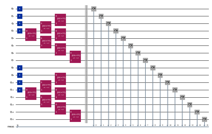
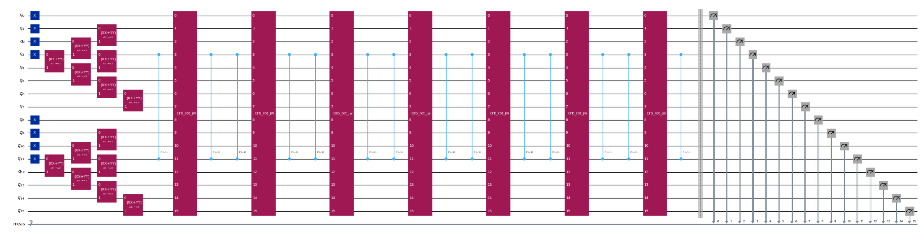
reference_energy, _ = pyscf.fci.direct_spin1.kernel(h1e, h2e, norb, nelec)

Next, we generate the circuits to produce the Krylov basis states. For each spin species, the initial state $\ket{\psi_0}$ is given by the superposition of all possible excitations of the three electrons closest to the Fermi level into the 4 closest empty modes starting from the state $|00\cdots 0011 \cdots 11\rangle$ , and realized by the application of seven XXPlusYYGates. The time-evolved states are produced by successive applications of a second-order Trotter step.

For a more detailed description of this model and how the circuits are designed, refer to "Quantum-Centric Algorithm for Sample-Based Krylov Diagonalization".

from typing import Sequence

import ffsim
import scipy
from qiskit import QuantumCircuit, QuantumRegister
from qiskit.circuit import CircuitInstruction, Qubit
from qiskit.circuit.library import CPhaseGate, XGate, XXPlusYYGate


def prepare_initial_state(qubits: Sequence[Qubit], norb: int, nocc: int):
    """Prepare initial state."""
    assert norb >= 8
    x_gate = XGate()
    rot = XXPlusYYGate(0.5 * np.pi, -0.5 * np.pi)
    for i in range(nocc):
        yield CircuitInstruction(x_gate, [qubits[i]])
        yield CircuitInstruction(x_gate, [qubits[norb + i]])
    for i in range(3):
        for j in range(nocc - i - 1, nocc + i, 2):
            yield CircuitInstruction(rot, [qubits[j], qubits[j + 1]])
            yield CircuitInstruction(
                rot, [qubits[norb + j], qubits[norb + j + 1]]
            )
    yield CircuitInstruction(rot, [qubits[j + 1], qubits[j + 2]])
    yield CircuitInstruction(
        rot, [qubits[norb + j + 1], qubits[norb + j + 2]]
    )


def trotter_step(
    qubits: Sequence[Qubit],
    time_step: float,
    one_body_evolution: np.ndarray,
    h2e: np.ndarray,
    impurity_index: int,
    norb: int,
):
    """A Trotter step."""
    # Assume the two-body interaction is just the on-site interaction of the impurity
    onsite = h2e[
        impurity_index, impurity_index, impurity_index, impurity_index
    ]
    # Two-body evolution for half the time
    yield CircuitInstruction(
        CPhaseGate(-0.5 * time_step * onsite),
        [qubits[impurity_index], qubits[norb + impurity_index]],
    )
    # One-body evolution for the full time
    yield CircuitInstruction(
        ffsim.qiskit.OrbitalRotationJW(norb, one_body_evolution), qubits
    )
    # Two-body evolution for half the time
    yield CircuitInstruction(
        CPhaseGate(-0.5 * time_step * onsite),
        [qubits[impurity_index], qubits[norb + impurity_index]],
    )


# Time step
time_step = 0.2
# Number of Krylov basis states
krylov_dim = 8

# Initialize circuit
qubits = QuantumRegister(2 * norb, name="q")
circuit = QuantumCircuit(qubits)

# Generate initial state
for instruction in prepare_initial_state(qubits, norb=norb, nocc=norb // 2):
    circuit.append(instruction)
circuit.measure_all()

# Create list of circuits, starting with the initial state circuit
circuits = [circuit.copy()]

# Add time evolution circuits to the list
one_body_evolution = scipy.linalg.expm(-1j * time_step * h1e_momentum)
for i in range(krylov_dim - 1):
    # Remove measurements
    circuit.remove_final_measurements()
    # Append another Trotter step
    for instruction in trotter_step(
        qubits,
        time_step,
        one_body_evolution,
        h2e_momentum,
        impurity_index,
        norb,
    ):
        circuit.append(instruction)
    # Measure qubits
    circuit.measure_all()
    # Add a copy of the circuit to the list
    circuits.append(circuit.copy())

circuits[0].draw("mpl", scale=0.4, fold=-1)

Output:

circuits[-1].draw("mpl", scale=0.4, fold=-1)

Output:

Step 2: Optimize problem for quantum execution

Next, we optimize the circuit for a target hardware. For now, we'll create a generic backend with a specified number of qubits and a gate set that the time evolution circuits naturally decompose to.

from qiskit.providers.fake_provider import GenericBackendV2

backend = GenericBackendV2(
    2 * norb, basis_gates=["cp", "xx_plus_yy", "p", "x"]
)

Now, we use Qiskit to transpile the circuits to the target backend.

from qiskit.transpiler import generate_preset_pass_manager

pass_manager = generate_preset_pass_manager(
    optimization_level=3, backend=backend
)
isa_circuits = pass_manager.run(circuits)

Step 3: Execute by using Qiskit primitives

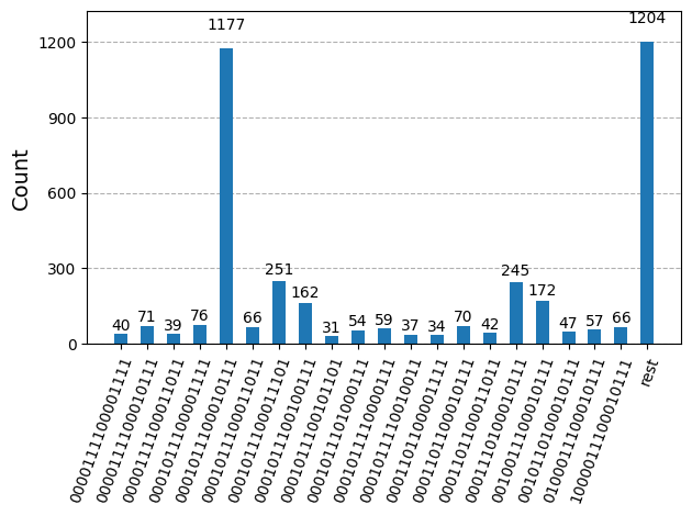
After optimizing the circuits for hardware execution, we are ready to run them on the target hardware and collect samples for ground state energy estimation. After using the Sampler primitive to sample bitstrings from each circuit, we combine all of the results into a single counts dictionary and plot the top 20 most commonly sampled bitstrings.

from qiskit.visualization import plot_histogram
from qiskit.primitives import StatevectorSampler

# Sample from the circuits
sampler = StatevectorSampler()
job = sampler.run(isa_circuits, shots=500)

Output:

/home/kjs/projects/documentation/.venv/lib/python3.12/site-packages/qiskit/circuit/quantumcircuit.py:4625: UserWarning: Trying to add QuantumRegister to a QuantumCircuit having a layout
  circ.add_register(qreg)

from qiskit.primitives import BitArray

# Combine the shots from the individual Trotter circuits
bit_array = BitArray.concatenate_shots(
    [result.data.meas for result in job.result()]
)

plot_histogram(bit_array.get_counts(), number_to_keep=20)

Output:

Step 4: Post-process and return result to desired classical format

Now, we run the SQD algorithm using the diagonalize_fermionic_hamiltonian function. See the API documentation for explanations of the arguments to this function.

from qiskit_addon_sqd.fermion import (
    SCIResult,
    diagonalize_fermionic_hamiltonian,
)

# List to capture intermediate results
result_history = []


def callback(results: list[SCIResult]):
    result_history.append(results)
    iteration = len(result_history)
    print(f"Iteration {iteration}")
    for i, result in enumerate(results):
        print(f"\tSubsample {i}")
        print(f"\t\tEnergy: {result.energy}")
        print(
            f"\t\tSubspace dimension: {np.prod(result.sci_state.amplitudes.shape)}"
        )


rng = np.random.default_rng(24)
result = diagonalize_fermionic_hamiltonian(
    h1e_momentum,
    h2e_momentum,
    bit_array,
    samples_per_batch=100,
    norb=norb,
    nelec=nelec,
    num_batches=3,
    max_iterations=5,
    symmetrize_spin=True,
    callback=callback,
    seed=rng,
)

Output:

Iteration 1
	Subsample 0
		Energy: -13.4222953188441
		Subspace dimension: 529
	Subsample 1
		Energy: -13.42237556285828
		Subspace dimension: 784
	Subsample 2
		Energy: -13.422045397387413
		Subspace dimension: 529
Iteration 2
	Subsample 0
		Energy: -13.422379583305478
		Subspace dimension: 900
	Subsample 1
		Energy: -13.422376197704326
		Subspace dimension: 841
	Subsample 2
		Energy: -13.422421162849295
		Subspace dimension: 1089
Iteration 3
	Subsample 0
		Energy: -13.422421164670345
		Subspace dimension: 1156
	Subsample 1
		Energy: -13.422421492737689
		Subspace dimension: 1156
	Subsample 2
		Energy: -13.422421205869572
		Subspace dimension: 1156
Iteration 4
	Subsample 0
		Energy: -13.422421494558726
		Subspace dimension: 1225
	Subsample 1
		Energy: -13.422421492737689
		Subspace dimension: 1156
	Subsample 2
		Energy: -13.422421492737689
		Subspace dimension: 1156

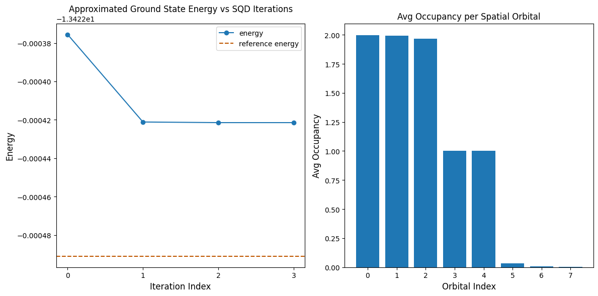
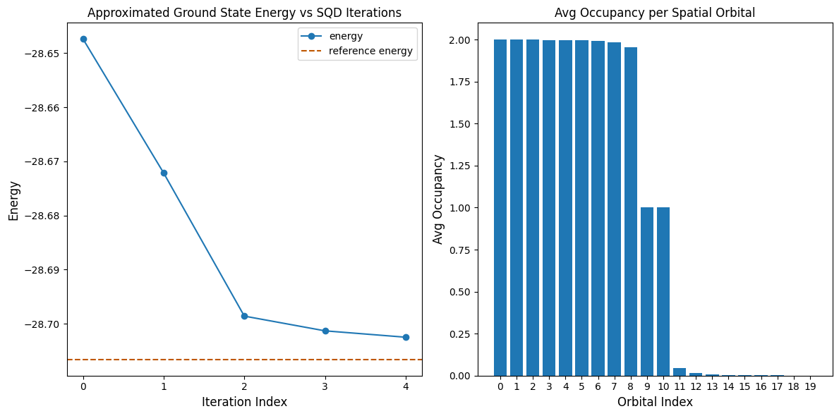
The following code cell plots the results. The first plot shows the computed energy as a function of the number of configuration recovery iterations, and the second plot shows the average occupancy of each spatial orbital after the final iteration. Since this is such a small problem, the first iteration already brings us very close to the exact energy (note the scale of the y axis).

import matplotlib.pyplot as plt

min_es = [
    min(result, key=lambda res: res.energy).energy
    for result in result_history
]
min_id, min_e = min(enumerate(min_es), key=lambda x: x[1])

# Data for energies plot
x1 = range(len(result_history))

# Data for avg spatial orbital occupancy
y2 = np.sum(result.orbital_occupancies, axis=0)
x2 = range(len(y2))

fig, axs = plt.subplots(1, 2, figsize=(12, 6))

# Plot energies
axs[0].plot(x1, min_es, label="energy", marker="o")
axs[0].set_xticks(x1)
axs[0].set_xticklabels(x1)
axs[0].axhline(
    y=reference_energy,
    color="#BF5700",
    linestyle="--",
    label="reference energy",
)
axs[0].set_title("Approximated Ground State Energy vs SQD Iterations")
axs[0].set_xlabel("Iteration Index", fontdict={"fontsize": 12})
axs[0].set_ylabel("Energy", fontdict={"fontsize": 12})
axs[0].legend()

# Plot orbital occupancy
axs[1].bar(x2, y2, width=0.8)
axs[1].set_xticks(x2)
axs[1].set_xticklabels(x2)
axs[1].set_title("Avg Occupancy per Spatial Orbital")
axs[1].set_xlabel("Orbital Index", fontdict={"fontsize": 12})
axs[1].set_ylabel("Avg Occupancy", fontdict={"fontsize": 12})

print(f"Reference energy: {reference_energy:.5f}")
print(f"SQD energy: {min_e:.5f}")
print(f"Absolute error: {abs(min_e - reference_energy):.5f}")
plt.tight_layout()
plt.show()

Output:

Reference energy: -13.42249
SQD energy: -13.42242
Absolute error: 0.00007

Verifying the energy

The energy returned by SQD is guaranteed to be an upper bound to the true ground state energy. The value of the energy can be verified because SQD also returns the coefficients of the state vector approximating the ground state. You can compute the energy from the state vector using its 1- and 2-particle reduced density matrices, as demonstrated in the following code cell.

rdm1 = result.sci_state.rdm(rank=1, spin_summed=True)
rdm2 = result.sci_state.rdm(rank=2, spin_summed=True)

energy = np.sum(h1e_momentum * rdm1) + 0.5 * np.sum(h2e_momentum * rdm2)

print(f"Recomputed energy: {energy:.5f}")

Output:

Recomputed energy: -13.42242

Large-scale hardware example

Now, we run a larger example on a real QPU. For the reference energy, we use the results of a DMRG calculation that was performed separately.

from qiskit_ibm_runtime import SamplerV2 as Sampler
from qiskit_ibm_runtime import QiskitRuntimeService

# Model parameters
norb = 20
nelec = (norb // 2, norb // 2)
n_bath = norb - 1
hybridization = 1.0
hopping = 1.0
onsite = 10.0
chemical_potential = -0.5 * onsite

# Generate Hamiltonian and orbital rotation
h1e, h2e = siam_hamiltonian(
    norb=norb,
    hopping=hopping,
    onsite=onsite,
    hybridization=hybridization,
    chemical_potential=chemical_potential,
)
orbital_rotation = momentum_basis(norb)
h1e_momentum, h2e_momentum = rotated(h1e, h2e, orbital_rotation.T.conj())
impurity_index = n_bath // 2

# Set reference energy to DMRG value computed separately
reference_energy = -28.70659686

# Algorithm parameters
time_step = 0.2
krylov_dim = 8

# Construct circuits
qubits = QuantumRegister(2 * norb, name="q")
circuit = QuantumCircuit(qubits)
for instruction in prepare_initial_state(qubits, norb=norb, nocc=norb // 2):
    circuit.append(instruction)
circuit.measure_all()
circuits = [circuit.copy()]
one_body_evolution = scipy.linalg.expm(-1j * time_step * h1e_momentum)
for i in range(krylov_dim - 1):
    circuit.remove_final_measurements()
    for instruction in trotter_step(
        qubits,
        time_step,
        one_body_evolution,
        h2e_momentum,
        impurity_index,
        norb,
    ):
        circuit.append(instruction)
    circuit.measure_all()
    circuits.append(circuit.copy())

# Initialize hardware backend
service = QiskitRuntimeService()
backend = service.least_busy(
    operational=True, simulator=False, min_num_qubits=127
)
print(f"Using backend {backend.name}")

# Transpile to backend
pass_manager = generate_preset_pass_manager(
    optimization_level=3, backend=backend
)
isa_circuits = pass_manager.run(circuits)

# Sample from the circuits
sampler = Sampler(backend)
job = sampler.run(isa_circuits, shots=500)

# Combine the shots from the individual Trotter circuits
bit_array = BitArray.concatenate_shots(
    [result.data.meas for result in job.result()]
)

# Run configuration recovery and diagonalization
result_history = []


def callback(results: list[SCIResult]):
    result_history.append(results)
    iteration = len(result_history)
    print(f"Iteration {iteration}")
    for i, result in enumerate(results):
        print(f"\tSubsample {i}")
        print(f"\t\tEnergy: {result.energy}")
        print(
            f"\t\tSubspace dimension: {np.prod(result.sci_state.amplitudes.shape)}"
        )


rng = np.random.default_rng(24)
result = diagonalize_fermionic_hamiltonian(
    h1e_momentum,
    h2e_momentum,
    bit_array,
    samples_per_batch=100,
    norb=norb,
    nelec=nelec,
    num_batches=3,
    max_iterations=5,
    symmetrize_spin=True,
    callback=callback,
    seed=rng,
)


# Plot results
min_es = [
    min(result, key=lambda res: res.energy).energy
    for result in result_history
]
min_id, min_e = min(enumerate(min_es), key=lambda x: x[1])
x1 = range(len(result_history))
y2 = np.sum(result.orbital_occupancies, axis=0)
x2 = range(len(y2))
fig, axs = plt.subplots(1, 2, figsize=(12, 6))
axs[0].plot(x1, min_es, label="energy", marker="o")
axs[0].set_xticks(x1)
axs[0].set_xticklabels(x1)
axs[0].axhline(
    y=reference_energy,
    color="#BF5700",
    linestyle="--",
    label="reference energy",
)
axs[0].set_title("Approximated Ground State Energy vs SQD Iterations")
axs[0].set_xlabel("Iteration Index", fontdict={"fontsize": 12})
axs[0].set_ylabel("Energy", fontdict={"fontsize": 12})
axs[0].legend()
axs[1].bar(x2, y2, width=0.8)
axs[1].set_xticks(x2)
axs[1].set_xticklabels(x2)
axs[1].set_title("Avg Occupancy per Spatial Orbital")
axs[1].set_xlabel("Orbital Index", fontdict={"fontsize": 12})
axs[1].set_ylabel("Avg Occupancy", fontdict={"fontsize": 12})
print(f"Reference energy: {reference_energy:.5f}")
print(f"SQD energy: {min_e:.5f}")
print(f"Absolute error: {abs(min_e - reference_energy):.5f}")
plt.tight_layout()
plt.show()

Output:

Using backend ibm_boston
Iteration 1
	Subsample 0
		Energy: -28.63965951544449
		Subspace dimension: 9801
	Subsample 1
		Energy: -28.625588929202006
		Subspace dimension: 9409
	Subsample 2
		Energy: -28.647371834135498
		Subspace dimension: 8281
Iteration 2
	Subsample 0
		Energy: -28.67213260849567
		Subspace dimension: 29584
	Subsample 1
		Energy: -28.670340686158816
		Subspace dimension: 27225
	Subsample 2
		Energy: -28.669976379525988
		Subspace dimension: 31329
Iteration 3
	Subsample 0
		Energy: -28.68622875601382
		Subspace dimension: 36100
	Subsample 1
		Energy: -28.698569623143126
		Subspace dimension: 34225
	Subsample 2
		Energy: -28.694848533971882
		Subspace dimension: 33856
Iteration 4
	Subsample 0
		Energy: -28.69883392844593
		Subspace dimension: 42025
	Subsample 1
		Energy: -28.701289495200996
		Subspace dimension: 38025
	Subsample 2
		Energy: -28.699319594978245
		Subspace dimension: 45369
Iteration 5
	Subsample 0
		Energy: -28.701936886834154
		Subspace dimension: 51076
	Subsample 1
		Energy: -28.702468711812013
		Subspace dimension: 53824
	Subsample 2
		Energy: -28.702298147575938
		Subspace dimension: 52900
Reference energy: -28.70660
SQD energy: -28.70247
Absolute error: 0.00413

Next steps

If you found this work interesting, you might be interested in the following material:

Recommendations

Sample-based quantum diagonalization of a chemistry Hamiltonian - a related tutorial using a heuristic variational ansatz instead of Trotter circuits
Krylov quantum diagonalization of lattice Hamiltonians - a tutorial on the KQD method
SQD addon API documentation - reference for the diagonalize_fermionic_hamiltonian function

Quantum-Centric Algorithm for Sample-Based Krylov Diagonalization - the paper this tutorial is based on