Sample-based quantum diagonalization of a chemistry Hamiltonian

Usage estimate: under one minute on a Heron r2 processor (NOTE: This is an estimate only. Your runtime might vary.)

Learning outcomes

After going through this tutorial, users should understand:

How to use the SQD Qiskit addon to approximate the ground state energy of a molecular system using bitstrings sampled from a quantum processing unit (QPU).
How to use ffsim to construct a local unitary cluster Jastrow (LUCJ) circuit for quantum chemistry simulation.

Prerequisites

We suggest that users are familiar with the following topics before going through this tutorial

Quantum chemistry and second quantization
Using the Sampler primitive to sample from quantum circuits

Background

In this tutorial, we show how to post-process noisy quantum samples to find an approximation to the ground state of the nitrogen molecule $\text{N}_2$ at equilibrium bond length, using the sample-based quantum diagonalization (SQD) algorithm, utilizing the SQD Qiskit addons. More details on the software can be found in the corresponding docs with a simple example to get started.

This tutorial is geared towards users who are familiar with quantum chemistry, familiarity with finding ground state energies of a molecule. If you would like a detailed walk through on the workflow, which explains please refer to our quantum diagonalization algorithm course.

SQD is a technique for finding eigenvalues and eigenvectors of quantum operators, such as a quantum system Hamiltonian, using quantum and distributed classical computing together. Classical distributed computing is used to process samples obtained from a quantum processor, and to project and diagonalize a target Hamiltonian in a subspace spanned by them. An SQD-based workflow has the following steps:

Choose a circuit ansatz and apply it on a quantum computer to a reference state (in this case, the Hartree-Fock state).
Sample bitstrings from the resulting quantum state.
Run the self-consistent configuration recovery procedure on the bitstrings to obtain the approximation to the ground state.

SQD is known to work well when the target eigenstate is sparse: the wave function is supported in a set of basis states $\mathcal{S} = \{|x\rangle \}$ whose size does not increase exponentially with the size of the problem.

Quantum chemistry

The Hamiltonian of a molecular system can be written as

\hat{H} = \sum_{ \substack{pr\\\sigma} } h_{pr} \, \hat{a}^\dagger_{p\sigma} \hat{a}_{r\sigma} + \frac12 \sum_{ \substack{prqs\\\sigma\tau} } h_{prqs} \, \hat{a}^\dagger_{p\sigma} \hat{a}^\dagger_{q\tau} \hat{a}_{s\tau} \hat{a}_{r\sigma},

where the $h_{pr}$ and $h_{prqs}$ are complex numbers called molecular integrals that can be calculated from the specification of the molecule using a computer program. In this tutorial, we compute the integrals using the PySCF software package.

For details about how the molecular Hamiltonian is derived, consult a textbook on quantum chemistry (for example, Modern Quantum Chemistry by Szabo and Ostlund). For a high-level explanation of how quantum chemistry problems are mapped onto quantum computers, check out the lecture Mapping Problems to Qubits from Qiskit Global Summer School 2024.

Local unitary cluster Jastrow (LUCJ) ansatz

SQD requires a quantum circuit ansatz to draw samples from. In this tutorial, we'll use the local unitary cluster Jastrow (LUCJ) ansatz due to its combination of physical motivation and hardware-friendliness. We'll use ffsim to construct the ansatz circuit.

The LUCJ ansatz adapts to QPUs with restricted qubit connectivity. The spin orbitals are mapped to qubits such that the ansatz does not require routing with SWAP gates. The IBM® hardware has a heavy-hex lattice qubit topology, in which case we can adopt a "zig-zag" pattern, depicted below. In this pattern, orbitals with the same spin are mapped to qubits with a line topology (red and blue circles), and a connection between orbitals of different spin is present at every 4th spatial orbital, with the connection being facilitated by an ancilla qubit (purple circles).

Qubit mapping diagram for the LUCJ ansatz on a heavy-hex lattice

Self-consistent configuration recovery

The self-consistent configuration recovery procedure is designed to extract as much signal as possible from noisy quantum samples. Because the molecular Hamiltonian conserves particle number and spin Z, it makes sense to choose a circuit ansatz that also conserves these symmetries. When applied to the Hartree-Fock state, the resulting state has a fixed particle number and spin Z in the noiseless setting. Therefore, the spin- $\alpha$ and spin- $\beta$ halves of any bitstring sampled from this state should have the same Hamming weight as in the Hartree-Fock state. Due to the presence of noise in current quantum processors, some measured bitstrings will violate this property. A simple form of postselection would discard these bitstrings, but this is wasteful because those bitstrings might still contain some signal. The self-consistent recovery procedure attempts to recover some of that signal in post-processing. The procedure is iterative and requires as input an estimate of the average occupancies of each orbital in the ground state, which is first computed from the raw samples. The procedure is run in a loop, and each iteration has the following steps:

For each bitstring that violates the specified symmetries, flip its bits with a probabilistic procedure designed to bring the bitstring closer to the current estimate of the average orbital occupancies, to obtain a new bitstring.
Collect all of the old and new bitstrings that satisfy the symmetries, and subsample subsets of a fixed size, chosen in advance.
For each subset of bitstrings, project the Hamiltonian into the subspace spanned by the corresponding basis vectors (see the previous section for a description of these basis vectors), and compute a ground state estimate of the projected Hamiltonian on a classical computer.
Update the estimate of the average orbital occupancies with the ground state estimate with the lowest energy.

SQD workflow diagram

The SQD workflow is depicted in the following diagram:

Requirements

Before starting this tutorial, ensure that you have the following installed:

Qiskit SDK v1.0 or later, with visualization support
Qiskit Runtime v0.22 or later (pip install qiskit-ibm-runtime)
SQD Qiskit addon v0.11 or later (pip install qiskit-addon-sqd)
ffsim v0.0.72 or later (pip install ffsim)

Setup

import math

import ffsim
import matplotlib.pyplot as plt
import numpy as np
import pyscf
import pyscf.cc
import pyscf.mcscf
from qiskit import QuantumCircuit, QuantumRegister
from qiskit.primitives import StatevectorSampler
from qiskit.providers.fake_provider import GenericBackendV2
from qiskit.transpiler.preset_passmanagers import generate_preset_pass_manager
from qiskit_ibm_runtime import QiskitRuntimeService
from qiskit_ibm_runtime import SamplerV2 as Sampler

Small-scale simulator example

In this tutorial, we will find an approximation to the ground state of a nitrogen molecule at equilibrium. We first use a small STO-6G basis set so that we can simulate the experiment and make sure it's working.

Step 1: Map classical inputs to a quantum problem

First, we specify the molecule and its properties.

# Specify molecule properties
open_shell = False
spin_sq = 0

# Build N2 molecule
mol = pyscf.gto.Mole()
mol.build(
    atom=[["N", (0, 0, 0)], ["N", (1.0, 0, 0)]],
    basis="sto-6g",
    symmetry="Dooh",
)

# Define active space
n_frozen = 2
active_space = range(n_frozen, mol.nao_nr())

# Get molecular integrals
scf = pyscf.scf.RHF(mol).run()
norb = len(active_space)
n_electrons = int(sum(scf.mo_occ[active_space]))
n_alpha = (n_electrons + mol.spin) // 2
n_beta = (n_electrons - mol.spin) // 2
nelec = (n_alpha, n_beta)
cas = pyscf.mcscf.CASCI(scf, norb, nelec)
mo = cas.sort_mo(active_space, base=0)
hcore, nuclear_repulsion_energy = cas.get_h1cas(mo)
eri = pyscf.ao2mo.restore(1, cas.get_h2cas(mo), norb)

# Compute exact energy using FCI
reference_energy = cas.run().e_tot

print(f"norb = {norb}")
print(f"nelec = {nelec}")

Output:

converged SCF energy = -108.464957764796
CASCI E = -108.595987350986  E(CI) = -32.4115475088426  S^2 = 0.0000000
norb = 8
nelec = (5, 5)

Before constructing the LUCJ ansatz circuit, we first perform a CCSD calculation in the following code cell. The $t_1$ and $t_2$ amplitudes from this calculation will be used to initialize the parameters of the ansatz.

# Get CCSD t2 amplitudes for initializing the ansatz
ccsd = pyscf.cc.CCSD(
    scf, frozen=[i for i in range(mol.nao_nr()) if i not in active_space]
).run()
t1 = ccsd.t1
t2 = ccsd.t2

Output:

E(CCSD) = -108.5933309085008  E_corr = -0.1283731437052352

Now, we use ffsim to create the ansatz circuit. Since our molecule has a closed-shell Hartree-Fock state, we use the spin-balanced variant of the UCJ ansatz, UCJOpSpinBalanced. We pass interaction pairs appropriate for a heavy-hex lattice qubit topology (see the background section on the LUCJ ansatz). We set optimize=True in the from_t_amplitudes method to enable the "compressed" double-factorization of the $t_2$ amplitudes (see The local unitary cluster Jastrow (LUCJ) ansatz at ffsim's documentation for details).

n_reps = 1
alpha_alpha_indices = [(p, p + 1) for p in range(norb - 1)]
alpha_beta_indices = [(p, p) for p in range(0, norb, 4)]


ucj_op = ffsim.UCJOpSpinBalanced.from_t_amplitudes(
    t2=t2,
    t1=t1,
    n_reps=n_reps,
    interaction_pairs=(alpha_alpha_indices, alpha_beta_indices),
    # Setting optimize=True enables the "compressed" factorization
    optimize=True,
    # Limit the number of optimization iterations to prevent the code cell from running
    # too long. Removing this line may improve results.
    options=dict(maxiter=1000),
)

# create an empty quantum circuit
qubits = QuantumRegister(2 * norb, name="q")
circuit = QuantumCircuit(qubits)

# prepare Hartree-Fock state as the reference state and append it to the quantum circuit
circuit.append(ffsim.qiskit.PrepareHartreeFockJW(norb, nelec), qubits)

# apply the UCJ operator to the reference state
circuit.append(ffsim.qiskit.UCJOpSpinBalancedJW(ucj_op), qubits)
circuit.measure_all()

Output:

WARNING:2026-03-25 16:00:12,333:jax._src.xla_bridge:850: An NVIDIA GPU may be present on this machine, but a CUDA-enabled jaxlib is not installed. Falling back to cpu.

Step 2: Optimize problem for quantum hardware execution

Next, we optimize the circuit for a target hardware. For now, we'll just create a generic backend with a specified number of qubits and a gate set that the LUCJ ansatz naturally decomposes to.

backend = GenericBackendV2(
    2 * norb, basis_gates=["cp", "xx_plus_yy", "p", "x"]
)

pass_manager = generate_preset_pass_manager(
    optimization_level=3, backend=backend
)
# Set the pre-initialization stage of the pass manager with passes suggested by ffsim
pass_manager.pre_init = ffsim.qiskit.PRE_INIT
isa_circuit = pass_manager.run(circuit)
print(f"Gate counts: {isa_circuit.count_ops()}")

Output:

Gate counts: OrderedDict({'xx_plus_yy': 86, 'cp': 16, 'p': 16, 'measure': 16, 'x': 10, 'barrier': 1})

Step 3: Execute using Qiskit primitives

After optimizing the circuit for hardware execution, we are ready to run it on the target hardware and collect samples for ground state energy estimation. As we only have one circuit, we will use Qiskit Runtime's Job execution mode and execute our circuit.

rng = np.random.default_rng()
sampler = StatevectorSampler(seed=rng)
job = sampler.run([isa_circuit], shots=100_000)

Output:

/home/kjs/projects/documentation/.venv/lib/python3.12/site-packages/qiskit/circuit/quantumcircuit.py:4625: UserWarning: Trying to add QuantumRegister to a QuantumCircuit having a layout
  circ.add_register(qreg)

primitive_result = job.result()
pub_result = primitive_result[0]

Step 4: Post-process and return result in desired classical format

A useful metric to judge the quality of the QPU output is the number of valid configurations returned. A valid configuration has the correct particle number and spin Z, which means that the right half of the bitstring has Hamming weight equal to the number of spin-up electrons, and the left half has Hamming weight equal to the number of spin-down electrons. The following cell computes the fraction of sampled configurations that are valid.

def is_valid_bitstring(
    bitstring: str, norb: int, nelec: tuple[int, int]
) -> bool:
    n_alpha, n_beta = nelec
    return (
        len(bitstring) == 2 * norb
        and bitstring[norb:].count("1") == n_alpha
        and bitstring[:norb].count("1") == n_beta
    )


bit_array = pub_result.data.meas
num_valid = sum(
    is_valid_bitstring(b, norb, nelec) for b in bit_array.get_bitstrings()
)
valid_fraction = num_valid / bit_array.num_shots
print(f"Fraction of sampled configurations that are valid: {valid_fraction}")

Output:

Fraction of sampled configurations that are valid: 1.0

All of the bitstrings are valid because we are sampling the circuit on a noiseless simulator. When running on a noisy QPU, the fraction will be smaller than one, but hopefully it will be larger than the fraction you would expect if the bitstrings were sampled uniformly at random, which is computed in the following cell.

expected_fraction_random = (
    math.comb(norb, n_alpha) * math.comb(norb, n_beta) / 2 ** (2 * norb)
)
print(
    f"Expected fraction of valid configurations from uniformly random bitstrings: {expected_fraction_random}"
)

Output:

Expected fraction of valid configurations from uniformly random bitstrings: 0.0478515625

Now, we estimate the ground state energy of the Hamiltonian using the diagonalize_fermionic_hamiltonian function. This function performs the self-consistent configuration recovery procedure to iteratively refine the noisy quantum samples to improve the energy estimate. We pass a callback function so that we can save the intermediate results for later analysis. See the API documentation for explanations of the arguments to diagonalize_fermionic_hamiltonian.

Here, we use the initial_occupancies argument to diagonalize_fermionic_hamiltonian to specify the Hartree-Fock configuration as the initial guess for the orbital occupancies in the ground state. This approach is sensible for systems where the ground state has significant support on the Hartree-Fock configuration, but it might not be appropriate in other situations, though more advanced computational methods might yield better initial guesses in those cases. Specifying initial_occupancies also allows configuration recovery to run even if no valid configurations were sampled, as may be the case when sampling a large circuit on a noisy QPU. Without this argument, the configuration recovery would fail and raise an error if no valid configurations were provided.

from functools import partial

from qiskit_addon_sqd.fermion import (
    SCIResult,
    diagonalize_fermionic_hamiltonian,
    solve_sci_batch,
)

# SQD options
energy_tol = 1e-3
occupancies_tol = 1e-3
max_iterations = 5

# Eigenstate solver options
num_batches = 3
samples_per_batch = 300
symmetrize_spin = True
carryover_threshold = 1e-4
max_cycle = 200

# Use the Hartree-Fock configuration as an initial guess for the orbital occupancies
initial_occupancies = (
    np.array([1] * n_alpha + [0] * (norb - n_alpha)),
    np.array([1] * n_beta + [0] * (norb - n_beta)),
)

# Pass options to the built-in eigensolver. If you just want to use the defaults,
# you can omit this step, in which case you would not specify the sci_solver argument
# in the call to diagonalize_fermionic_hamiltonian below.
sci_solver = partial(solve_sci_batch, spin_sq=0.0, max_cycle=max_cycle)

# List to capture intermediate results
result_history = []


def callback(results: list[SCIResult]):
    result_history.append(results)
    iteration = len(result_history)
    print(f"Iteration {iteration}")
    for i, result in enumerate(results):
        print(f"\tSubsample {i}")
        print(f"\t\tEnergy: {result.energy + nuclear_repulsion_energy}")
        print(
            f"\t\tSubspace dimension: {np.prod(result.sci_state.amplitudes.shape)}"
        )


result = diagonalize_fermionic_hamiltonian(
    hcore,
    eri,
    bit_array,
    samples_per_batch=samples_per_batch,
    norb=norb,
    nelec=nelec,
    num_batches=num_batches,
    energy_tol=energy_tol,
    occupancies_tol=occupancies_tol,
    max_iterations=max_iterations,
    sci_solver=sci_solver,
    symmetrize_spin=symmetrize_spin,
    initial_occupancies=initial_occupancies,
    carryover_threshold=carryover_threshold,
    callback=callback,
    seed=rng,
)

final_energy = result.energy + nuclear_repulsion_energy
energy_error = final_energy - reference_energy
print(f"Final energy: {final_energy}")
print(f"Final energy error: {energy_error}")

Output:

Iteration 1
	Subsample 0
		Energy: -108.59570174319286
		Subspace dimension: 1849
	Subsample 1
		Energy: -108.59570174319286
		Subspace dimension: 1849
	Subsample 2
		Energy: -108.59570174319286
		Subspace dimension: 1849
Iteration 2
	Subsample 0
		Energy: -108.59570174319286
		Subspace dimension: 1849
	Subsample 1
		Energy: -108.59570174319286
		Subspace dimension: 1849
	Subsample 2
		Energy: -108.59570174319286
		Subspace dimension: 1849
Final energy: -108.59570174319286
Final energy error: 0.0002856077932023027

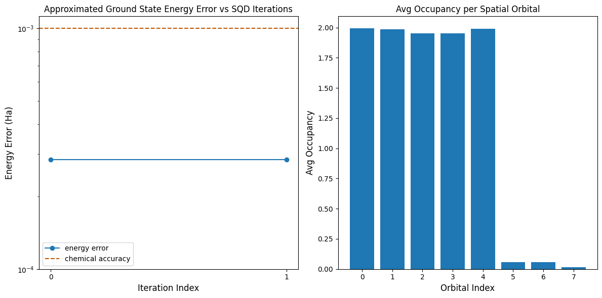
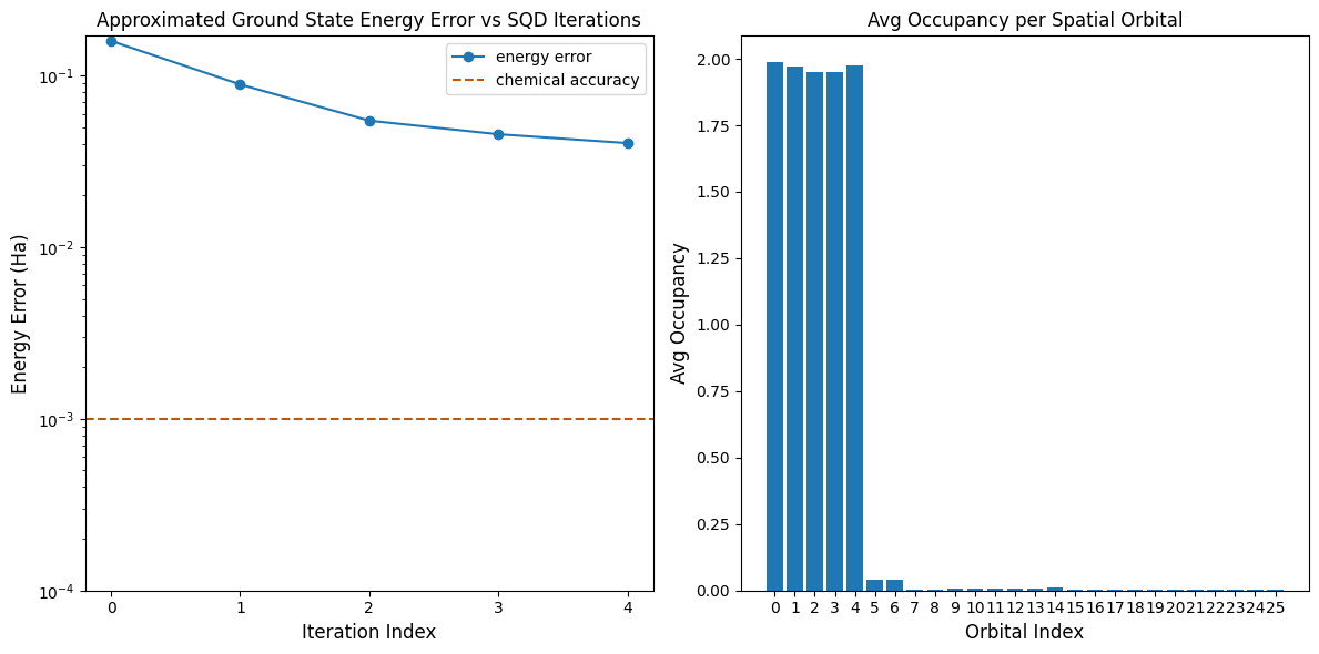
Visualize the results

The first plot shows that in this simulation, we are already within 1 mH of the exact answer after the first iteration (chemical accuracy is typically accepted to be 1 kcal/mol $\approx$ 1.6 mH). This is a small system, though, and because the samples are noiseless, configuration recovery is actually not needed. On a larger system run on a noisy QPU, multiple iterations of configuration recovery may be needed, and the final accuracy might be worse. Generally, the energy can be improved by allowing more iterations of configuration recovery or increasing the number of samples per batch.

The second plot shows the average occupancy of each spatial orbital after the final iteration. We can see that both the spin-up and spin-down electrons occupy the first five orbitals with high probability in our solutions.

# Data for energies plot
x1 = range(len(result_history))
min_e = [
    min(result, key=lambda res: res.energy).energy + nuclear_repulsion_energy
    for result in result_history
]
e_diff = [abs(e - reference_energy) for e in min_e]
yt1 = [1.0, 1e-1, 1e-2, 1e-3, 1e-4]

# Chemical accuracy (+/- 1 milli-Hartree)
chem_accuracy = 0.001

# Data for avg spatial orbital occupancy
y2 = np.sum(result.orbital_occupancies, axis=0)
x2 = range(len(y2))

fig, axs = plt.subplots(1, 2, figsize=(12, 6))

# Plot energies
axs[0].plot(x1, e_diff, label="energy error", marker="o")
axs[0].set_xticks(x1)
axs[0].set_xticklabels(x1)
axs[0].set_yticks(yt1)
axs[0].set_yticklabels(yt1)
axs[0].set_yscale("log")
axs[0].set_ylim(1e-4)
axs[0].axhline(
    y=chem_accuracy,
    color="#BF5700",
    linestyle="--",
    label="chemical accuracy",
)
axs[0].set_title("Approximated Ground State Energy Error vs SQD Iterations")
axs[0].set_xlabel("Iteration Index", fontdict={"fontsize": 12})
axs[0].set_ylabel("Energy Error (Ha)", fontdict={"fontsize": 12})
axs[0].legend()

# Plot orbital occupancy
axs[1].bar(x2, y2, width=0.8)
axs[1].set_xticks(x2)
axs[1].set_xticklabels(x2)
axs[1].set_title("Avg Occupancy per Spatial Orbital")
axs[1].set_xlabel("Orbital Index", fontdict={"fontsize": 12})
axs[1].set_ylabel("Avg Occupancy", fontdict={"fontsize": 12})

plt.tight_layout()
plt.show()

Output:

Large-scale hardware example

Now, we run a larger example on real quantum hardware. Here, we'll derive an active space for the nitrogen molecule from the cc-pVDZ basis set.

When executing the LUCJ circuit on hardware, care should be taken about how to map the qubits onto the hardware to minimize the overhead of qubit routing with SWAP gates. We recommend the following steps to optimize the ansatz and make it hardware-compatible.

Select physical qubits (initial_layout) from the target hardware that adheres to the "zig-zag" pattern described previously. Laying out qubits in this pattern leads to an efficient hardware-compatible circuit with less gates. Here, we include some code to automate the selection of the "zig-zag" pattern that uses a scoring heuristic to minimize the errors associated with the selected layout.
Generate a staged pass manager using the generate_preset_pass_manager function from qiskit with your choice of backend and initial_layout.
Set the pre_init stage of your staged pass manager to ffsim.qiskit.PRE_INIT. ffsim.qiskit.PRE_INIT includes qiskit transpiler passes that decompose gates into orbital rotations and then merges the orbital rotations, resulting in fewer gates in the final circuit.
Run the pass manager on your circuit.

Code for automated selection of "zig-zag" layout

from typing import Sequence

import rustworkx
from qiskit.providers import BackendV2
from rustworkx import NoEdgeBetweenNodes, PyGraph

IBM_TWO_Q_GATES = {"cx", "ecr", "cz"}


def create_linear_chains(num_orbitals: int) -> PyGraph:
    """In zig-zag layout, there are two linear chains (with connecting qubits between
    the chains). This function creates those two linear chains: a rustworkx PyGraph
    with two disconnected linear chains. Each chain contains `num_orbitals` number
    of nodes, that is, in the final graph there are `2 * num_orbitals` number of nodes.

    Args:
        num_orbitals (int): Number orbitals or nodes in each linear chain. They are
            also known as alpha-alpha interaction qubits.

    Returns:
        A rustworkx.PyGraph with two disconnected linear chains each with `num_orbitals`
            number of nodes.
    """
    G = rustworkx.PyGraph()

    for n in range(num_orbitals):
        G.add_node(n)

    for n in range(num_orbitals - 1):
        G.add_edge(n, n + 1, None)

    for n in range(num_orbitals, 2 * num_orbitals):
        G.add_node(n)

    for n in range(num_orbitals, 2 * num_orbitals - 1):
        G.add_edge(n, n + 1, None)

    return G


def create_lucj_zigzag_layout(
    num_orbitals: int, backend_coupling_graph: PyGraph
) -> tuple[PyGraph, int]:
    """This function creates the complete zigzag graph that 'can be mapped' to an IBM QPU with
    heavy-hex connectivity (the zigzag must be an isomorphic sub-graph to the QPU/backend
    coupling graph for it to be mapped).
    The zigzag pattern includes both linear chains (alpha-alpha interactions) and connecting
    qubits between the linear chains (alpha-beta interactions).

    Args:
        num_orbitals (int): Number of orbitals, that is, number of nodes in each alpha-alpha linear chain.
        backend_coupling_graph (PyGraph): The coupling graph of the backend on which the LUCJ ansatz
            will be mapped and run. This function takes the coupling graph as a undirected
            `rustworkx.PyGraph` where there is only one 'undirected' edge between two nodes,
            that is, qubits. Usually, the coupling graph of a IBM backend is directed (for example, Eagle devices
            such as ibm_brisbane) or may have two edges between two nodes (for example, Heron `ibm_torino`).
            A user needs to be make such graphs undirected and/or remove duplicate edges to make them
            compatible with this function.

    Returns:
        G_new (PyGraph): The graph with IBM backend compliant zigzag pattern.
        num_alpha_beta_qubits (int): Number of connecting qubits between the linear chains
            in the zigzag pattern. While we want as many connecting (alpha-beta) qubits between
            the linear (alpha-alpha) chains, we cannot accommodate all due to qubit and connectivity
            constraints of backends. This is the maximum number of connecting qubits the zigzag pattern
            can have while being backend compliant (that is, isomorphic to backend coupling graph).
    """
    isomorphic = False
    G = create_linear_chains(num_orbitals=num_orbitals)

    num_iters = num_orbitals
    while not isomorphic:
        G_new = G.copy()
        num_alpha_beta_qubits = 0
        for n in range(num_iters):
            if n % 4 == 0:
                new_node = 2 * num_orbitals + num_alpha_beta_qubits
                G_new.add_node(new_node)
                G_new.add_edge(n, new_node, None)
                G_new.add_edge(new_node, n + num_orbitals, None)
                num_alpha_beta_qubits = num_alpha_beta_qubits + 1
        isomorphic = rustworkx.is_subgraph_isomorphic(
            backend_coupling_graph, G_new
        )
        num_iters -= 1

    return G_new, num_alpha_beta_qubits


def lightweight_layout_error_scoring(
    backend: BackendV2,
    virtual_edges: Sequence[Sequence[int]],
    physical_layouts: Sequence[int],
    two_q_gate_name: str,
) -> list[list[list[int], float]]:
    """Lightweight and heuristic function to score isomorphic layouts. There can be many zigzag patterns,
    each with different set of physical qubits, that can be mapped to a backend. Some of them may
    include less noise qubits and couplings than others. This function computes a simple error score
    for each such layout. It sums up 2Q gate error for all couplings in the zigzag pattern (layout) and
    measurement of errors of physical qubits in the layout to compute the error score.

    Note:
        This lightweight scoring can be refined using concepts such as mapomatic.

    Args:
        backend (BackendV2): A backend.
        virtual_edges (Sequence[Sequence[int]]): Edges in the device compliant zigzag pattern where
            nodes are numbered from 0 to (2 * num_orbitals + num_alpha_beta_qubits).
        physical_layouts (Sequence[int]): All physical layouts of the zigzag pattern that are isomorphic
            to each other and to the larger backend coupling map.
        two_q_gate_name (str): The name of the two-qubit gate of the backend. The name is used for fetching
            two-qubit gate error from backend properties.

    Returns:
        scores (list): A list of lists where each sublist contains two items. First item is the layout, and
            second item is a float representing error score of the layout. The layouts in the `scores` are
            sorted in the ascending order of error score.
    """
    props = backend.properties()
    scores = []
    for layout in physical_layouts:
        total_2q_error = 0
        for edge in virtual_edges:
            physical_edge = (layout[edge[0]], layout[edge[1]])
            try:
                ge = props.gate_error(two_q_gate_name, physical_edge)
            except Exception:
                ge = props.gate_error(two_q_gate_name, physical_edge[::-1])
            total_2q_error += ge
        total_measurement_error = 0
        for qubit in layout:
            meas_error = props.readout_error(qubit)
            total_measurement_error += meas_error
        scores.append([layout, total_2q_error + total_measurement_error])

    return sorted(scores, key=lambda x: x[1])


def _make_backend_cmap_pygraph(backend: BackendV2) -> PyGraph:
    graph = backend.coupling_map.graph
    if not graph.is_symmetric():
        graph.make_symmetric()
    backend_coupling_graph = graph.to_undirected()

    edge_list = backend_coupling_graph.edge_list()
    removed_edge = []
    for edge in edge_list:
        if set(edge) in removed_edge:
            continue
        try:
            backend_coupling_graph.remove_edge(edge[0], edge[1])
            removed_edge.append(set(edge))
        except NoEdgeBetweenNodes:
            pass

    return backend_coupling_graph


def get_zigzag_physical_layout(
    num_orbitals: int, backend: BackendV2, score_layouts: bool = True
) -> tuple[list[int], int]:
    """The main function that generates the zigzag pattern with physical qubits that can be used
    as an `intial_layout` in a preset passmanager/transpiler.

    Args:
        num_orbitals (int): Number of orbitals.
        backend (BackendV2): A backend.
        score_layouts (bool): Optional. If `True`, it uses the `lightweight_layout_error_scoring`
            function to score the isomorphic layouts and returns the layout with less erroneous qubits.
            If `False`, returns the first isomorphic subgraph.

    Returns:
        A tuple of device compliant layout (list[int]) with zigzag pattern and an int representing
            number of alpha-beta-interactions.
    """
    backend_coupling_graph = _make_backend_cmap_pygraph(backend=backend)

    G, num_alpha_beta_qubits = create_lucj_zigzag_layout(
        num_orbitals=num_orbitals,
        backend_coupling_graph=backend_coupling_graph,
    )

    isomorphic_mappings = rustworkx.vf2_mapping(
        backend_coupling_graph, G, subgraph=True
    )
    isomorphic_mappings = list(isomorphic_mappings)

    edges = list(G.edge_list())

    layouts = []
    for mapping in isomorphic_mappings:
        initial_layout = [None] * (2 * num_orbitals + num_alpha_beta_qubits)
        for key, value in mapping.items():
            initial_layout[value] = key
        layouts.append(initial_layout)

    two_q_gate_name = IBM_TWO_Q_GATES.intersection(
        backend.configuration().basis_gates
    ).pop()

    if score_layouts:
        scores = lightweight_layout_error_scoring(
            backend=backend,
            virtual_edges=edges,
            physical_layouts=layouts,
            two_q_gate_name=two_q_gate_name,
        )

        return scores[0][0][:-num_alpha_beta_qubits], num_alpha_beta_qubits

    return layouts[0][:-num_alpha_beta_qubits], num_alpha_beta_qubits

Steps 1-4

Here we now put all the steps together into a singular workflow at a larger scale, which is then run on real quantum hardware.

# ------------------------------ Step 1 ------------------------------
# Build N2 molecule
mol = pyscf.gto.Mole()
mol.build(
    atom=[["N", (0, 0, 0)], ["N", (1.0, 0, 0)]],
    basis="cc-pvdz",
    symmetry="Dooh",
)

# Define active space
n_frozen = 2
active_space = range(n_frozen, mol.nao_nr())

# Get molecular integrals
scf = pyscf.scf.RHF(mol).run()
norb = len(active_space)
n_electrons = int(sum(scf.mo_occ[active_space]))
n_alpha = (n_electrons + mol.spin) // 2
n_beta = (n_electrons - mol.spin) // 2
nelec = (n_alpha, n_beta)
cas = pyscf.mcscf.CASCI(scf, norb, nelec)
mo = cas.sort_mo(active_space, base=0)
hcore, nuclear_repulsion_energy = cas.get_h1cas(mo)
eri = pyscf.ao2mo.restore(1, cas.get_h2cas(mo), norb)

# Store reference energy from SCI calculation performed separately
reference_energy = -109.22802921665716

print(f"norb = {norb}")
print(f"nelec = {nelec}")

# Get CCSD t2 amplitudes for initializing the ansatz
ccsd = pyscf.cc.CCSD(
    scf, frozen=[i for i in range(mol.nao_nr()) if i not in active_space]
).run()
t1 = ccsd.t1
t2 = ccsd.t2
n_reps = 1
alpha_alpha_indices = [(p, p + 1) for p in range(norb - 1)]
alpha_beta_indices = [(p, p) for p in range(0, norb, 4)]


ucj_op = ffsim.UCJOpSpinBalanced.from_t_amplitudes(
    t2=t2,
    t1=t1,
    n_reps=n_reps,
    interaction_pairs=(alpha_alpha_indices, alpha_beta_indices),
    # Setting optimize=True enables the "compressed" factorization
    optimize=True,
    # Limit the number of optimization iterations to prevent the code cell from running
    # too long. Removing this line may improve results.
    options=dict(maxiter=1000),
)


# create an empty quantum circuit
qubits = QuantumRegister(2 * norb, name="q")
circuit = QuantumCircuit(qubits)

# prepare Hartree-Fock state as the reference state and append it to the quantum circuit
circuit.append(ffsim.qiskit.PrepareHartreeFockJW(norb, nelec), qubits)

# apply the UCJ operator to the reference state
circuit.append(ffsim.qiskit.UCJOpSpinBalancedJW(ucj_op), qubits)
circuit.measure_all()


# ------------------------------ Step 2 ------------------------------

service = QiskitRuntimeService()
backend = service.least_busy(
    operational=True, simulator=False, min_num_qubits=133
)

print(f"Using backend {backend.name}")
initial_layout, _ = get_zigzag_physical_layout(norb, backend=backend)

pass_manager = generate_preset_pass_manager(
    optimization_level=3, backend=backend, initial_layout=initial_layout
)
pass_manager.pre_init = ffsim.qiskit.PRE_INIT
isa_circuit = pass_manager.run(circuit)

print(f"Gate counts: {isa_circuit.count_ops()}")


# ------------------------------ Step 3 ------------------------------
sampler = Sampler(mode=backend)
job = sampler.run([isa_circuit], shots=100_000)
primitive_result = job.result()
pub_result = primitive_result[0]


# ------------------------------ Step 4 ------------------------------

bit_array = pub_result.data.meas
num_valid = sum(
    is_valid_bitstring(b, norb, nelec) for b in bit_array.get_bitstrings()
)
valid_fraction = num_valid / bit_array.num_shots
print(f"Fraction of sampled configurations that are valid: {valid_fraction}")
expected_fraction_random = (
    math.comb(norb, n_alpha) * math.comb(norb, n_beta) / 2 ** (2 * norb)
)
print(
    f"Expected fraction of valid configurations from uniformly random bitstrings: {expected_fraction_random}"
)
# SQD options
energy_tol = 1e-3
occupancies_tol = 1e-3
max_iterations = 5

# Eigenstate solver options
num_batches = 3
samples_per_batch = 300
symmetrize_spin = True
carryover_threshold = 1e-4
max_cycle = 200

# Use the Hartree-Fock configuration as an initial guess for the orbital occupancies
initial_occupancies = (
    np.array([1] * n_alpha + [0] * (norb - n_alpha)),
    np.array([1] * n_beta + [0] * (norb - n_beta)),
)

# Pass options to the built-in eigensolver. If you just want to use the defaults,
# you can omit this step, in which case you would not specify the sci_solver argument
# in the call to diagonalize_fermionic_hamiltonian below.
sci_solver = partial(solve_sci_batch, spin_sq=0.0, max_cycle=max_cycle)

# List to capture intermediate results
result_history = []


result = diagonalize_fermionic_hamiltonian(
    hcore,
    eri,
    bit_array,
    samples_per_batch=samples_per_batch,
    norb=norb,
    nelec=nelec,
    num_batches=num_batches,
    energy_tol=energy_tol,
    occupancies_tol=occupancies_tol,
    max_iterations=max_iterations,
    sci_solver=sci_solver,
    symmetrize_spin=symmetrize_spin,
    initial_occupancies=initial_occupancies,
    carryover_threshold=carryover_threshold,
    callback=callback,
    seed=rng,
)

final_energy = result.energy + nuclear_repulsion_energy
energy_error = final_energy - reference_energy
print(f"Final energy: {final_energy}")
print(f"Final energy error: {energy_error}")

# Data for energies plot
x1 = range(len(result_history))
min_e = [
    min(result, key=lambda res: res.energy).energy + nuclear_repulsion_energy
    for result in result_history
]
e_diff = [abs(e - reference_energy) for e in min_e]
yt1 = [1.0, 1e-1, 1e-2, 1e-3, 1e-4]

# Chemical accuracy (+/- 1 milli-Hartree)
chem_accuracy = 0.001

# Data for avg spatial orbital occupancy
y2 = np.sum(result.orbital_occupancies, axis=0)
x2 = range(len(y2))

fig, axs = plt.subplots(1, 2, figsize=(12, 6))

# Plot energies
axs[0].plot(x1, e_diff, label="energy error", marker="o")
axs[0].set_xticks(x1)
axs[0].set_xticklabels(x1)
axs[0].set_yticks(yt1)
axs[0].set_yticklabels(yt1)
axs[0].set_yscale("log")
axs[0].set_ylim(1e-4)
axs[0].axhline(
    y=chem_accuracy,
    color="#BF5700",
    linestyle="--",
    label="chemical accuracy",
)
axs[0].set_title("Approximated Ground State Energy Error vs SQD Iterations")
axs[0].set_xlabel("Iteration Index", fontdict={"fontsize": 12})
axs[0].set_ylabel("Energy Error (Ha)", fontdict={"fontsize": 12})
axs[0].legend()

# Plot orbital occupancy
axs[1].bar(x2, y2, width=0.8)
axs[1].set_xticks(x2)
axs[1].set_xticklabels(x2)
axs[1].set_title("Avg Occupancy per Spatial Orbital")
axs[1].set_xlabel("Orbital Index", fontdict={"fontsize": 12})
axs[1].set_ylabel("Avg Occupancy", fontdict={"fontsize": 12})

plt.tight_layout()
plt.show()

Output:

converged SCF energy = -108.929838385609
norb = 26
nelec = (5, 5)
E(CCSD) = -109.2177884185543  E_corr = -0.2879500329450042
Using backend ibm_fez
Gate counts: OrderedDict({'sx': 7070, 'rz': 7004, 'cz': 1874, 'x': 52, 'measure': 52, 'barrier': 1})
Fraction of sampled configurations that are valid: 0.00018
Expected fraction of valid configurations from uniformly random bitstrings: 9.607888706852918e-07
Iteration 1
	Subsample 0
		Energy: -109.06896153670648
		Subspace dimension: 281961
	Subsample 1
		Energy: -109.02861595000536
		Subspace dimension: 263169
	Subsample 2
		Energy: -109.03904563251682
		Subspace dimension: 288369
Iteration 2
	Subsample 0
		Energy: -109.13773131837928
		Subspace dimension: 419904
	Subsample 1
		Energy: -109.11957805994658
		Subspace dimension: 404496
	Subsample 2
		Energy: -109.13928526896287
		Subspace dimension: 405769
Iteration 3
	Subsample 0
		Energy: -109.17341837077211
		Subspace dimension: 603729
	Subsample 1
		Energy: -109.16337313138857
		Subspace dimension: 579121
	Subsample 2
		Energy: -109.17116470035694
		Subspace dimension: 582169
Iteration 4
	Subsample 0
		Energy: -109.1805148352
		Subspace dimension: 769129
	Subsample 1
		Energy: -109.17712191946752
		Subspace dimension: 801025
	Subsample 2
		Energy: -109.18252582523913
		Subspace dimension: 776161
Iteration 5
	Subsample 0
		Energy: -109.18759713210412
		Subspace dimension: 976144
	Subsample 1
		Energy: -109.18538156651687
		Subspace dimension: 986049
	Subsample 2
		Energy: -109.18622955530022
		Subspace dimension: 1022121
Final energy: -109.18759713210412
Final energy error: 0.040432084553046366

Next steps

If you found this work interesting, you might be interested in the following material: