Quantum approximate optimization algorithm

Usage estimate: 22 minutes on a Heron r3 processor (NOTE: This is an estimate only. Your runtime might vary.)

Learning outcomes

After completing this tutorial, you can expect to understand the following information:

How to map a classical combinatorial optimization problem (max-cut) to a quantum Hamiltonian
How to implement and run the Quantum Approximate Optimization Algorithm (QAOA) using Qiskit Runtime sessions
How to scale a QAOA workflow from a small simulator example to utility-scale hardware execution

Prerequisites

It is recommended that you familiarize yourself with these topics:

Basics of quantum circuits
Variational algorithms
QAOA in depth — for a comprehensive treatment of the QAOA algorithm and applying it at utility scale

Background

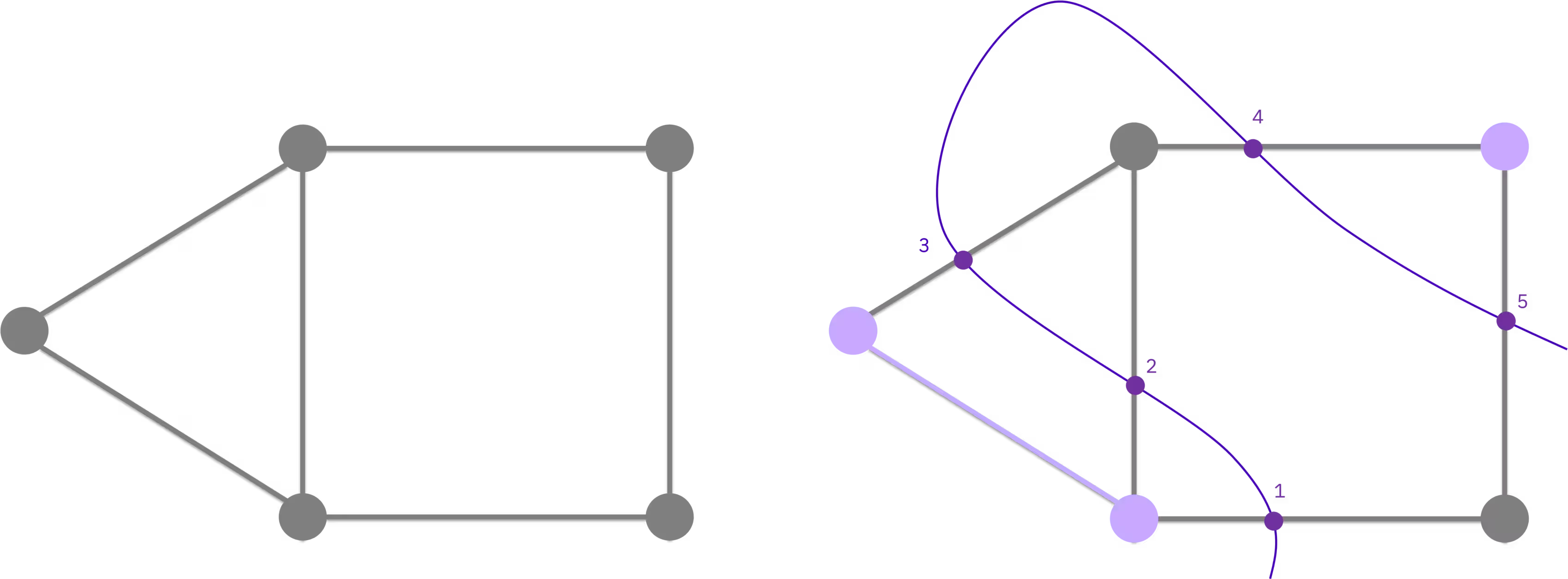
The Quantum Approximate Optimization Algorithm (QAOA) is a hybrid quantum-classical iterative method for solving combinatorial optimization problems. In this tutorial, you will use QAOA to solve the maximum-cut (max-cut) problem — an NP-hard optimization problem with applications in clustering, network science, and statistical physics. Given a graph of nodes connected by edges, the goal is to partition the nodes into two sets such that the number of edges crossing the partition is maximized.

From classical optimization to quantum circuits

Max-cut can be expressed as a classical binary optimization problem. Each node is assigned a binary variable $x_i \in \{0, 1\}$ indicating which set it belongs to. The objective is to maximize the number of edges where the endpoints are in different sets:

\max_{x \in \{0,1\}^n} \sum_{(i,j)} x_i + x_j - 2x_ix_j.

This is equivalently a Quadratic Unconstrained Binary Optimization (QUBO) problem of the form $\min_x\, x^T Q x$ . Through a standard variable substitution ( $x_i \to (1 - Z_i)/2$ ), the QUBO can be rewritten as a cost Hamiltonian whose ground state encodes the optimal solution. In general, this Hamiltonian has both quadratic and linear terms:

H_C = \sum_{ij} Q_{ij} \, Z_i Z_j + \sum_i b_i \, Z_i.

For the unweighted max-cut problem considered here, the linear coefficients vanish ( $b_i = 0$ ) and $Q_{ij} = 1$ for each edge, leaving the simpler form $H_C = \sum_{(i,j) \in E} Z_i Z_j$ that you will build in code below. The more general form above is what you would need to adapt this workflow to weighted graphs or other QUBO-expressible problems.

How QAOA works

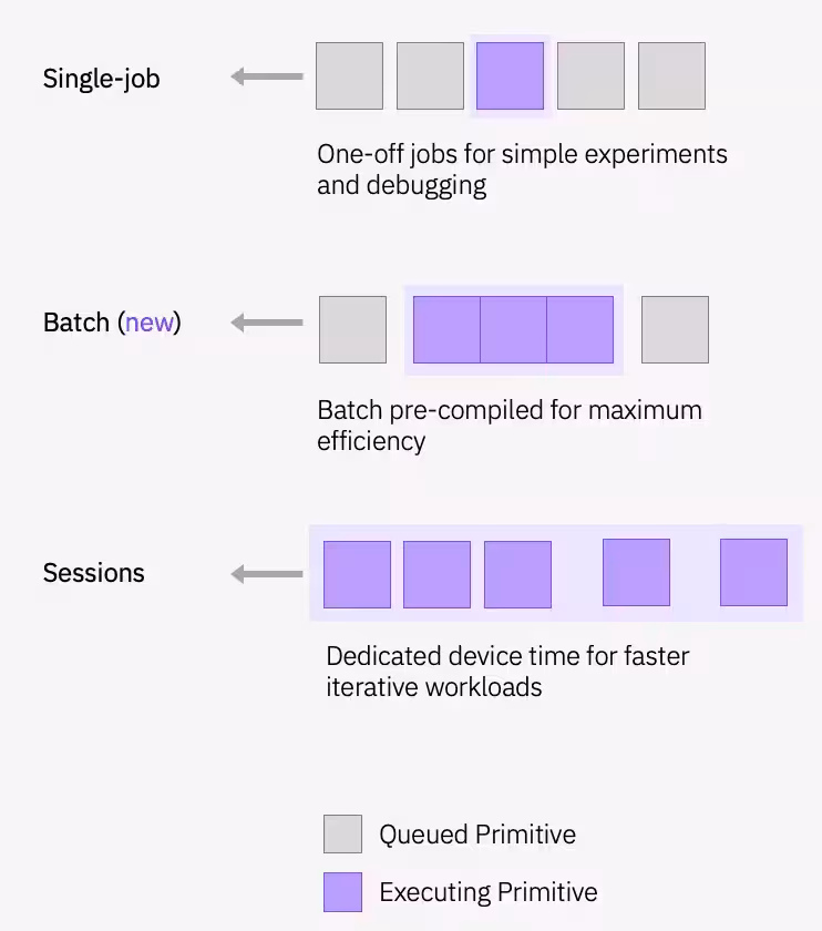
QAOA prepares candidate solutions by applying alternating layers of two operators to an initial superposition state $H^{\otimes n}|0\rangle$ : the cost operator $e^{-i\gamma_k H_C}$ and a mixer operator $e^{-i\beta_k H_m}$ . The angles $\gamma_k$ and $\beta_k$ are optimized in a classical feedback loop; the quantum computer evaluates the cost function, and a classical optimizer updates the parameters until convergence. This iterative loop runs within a Qiskit Runtime session, which keeps the quantum device reserved across iterations for lower latency.

For a deeper treatment of QAOA theory, including the full QUBO-to-Hamiltonian derivation, see the QAOA course module.

In this tutorial you will first solve max-cut on a small five-node graph, then scale the same workflow to a 100-node utility-scale problem on real hardware. Note on plan access: This tutorial uses Qiskit Runtime sessions, which are only available on the Premium Plan. If you are on the Open Plan, you cannot run this tutorial as written; instead, you will need to swap Session for job mode (as in, submit each iteration as an independent job rather than wrapping the optimization loop in with Session(...)). The workflow still runs, but each iteration incurs the full queue latency rather than reusing a reserved device. See Overview of available plans for more information.

Requirements

Before starting this tutorial, be sure you have the following installed:

Qiskit SDK v2.0 or later, with visualization support
Qiskit Runtime v0.22 or later (pip install qiskit-ibm-runtime)

In addition, you will need access to an instance on IBM Quantum® Platform.

Setup

import matplotlib.pyplot as plt
import rustworkx as rx
from rustworkx.visualization import mpl_draw as draw_graph
import numpy as np
from scipy.optimize import minimize
from collections import defaultdict
from typing import Sequence


from qiskit.quantum_info import SparsePauliOp
from qiskit.circuit.library import QAOAAnsatz
from qiskit.transpiler.preset_passmanagers import generate_preset_pass_manager

from qiskit_ibm_runtime import QiskitRuntimeService
from qiskit_ibm_runtime import Session, EstimatorV2 as Estimator
from qiskit_ibm_runtime import SamplerV2 as Sampler

Small-scale example

This section walks through each step of the QAOA workflow on a small five-node max-cut instance. Despite the "small-scale" label, this example still runs on real IBM Quantum hardware — the code selects a backend with 127 or more qubits and executes the circuit there.

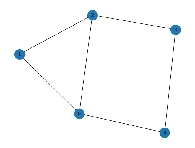
Initialize your problem by creating a graph with $n=5$ nodes.

n_small = 5

graph = rx.PyGraph()
graph.add_nodes_from(np.arange(0, n_small, 1))
edge_list = [
    (0, 1, 1.0),
    (0, 2, 1.0),
    (0, 4, 1.0),
    (1, 2, 1.0),
    (2, 3, 1.0),
    (3, 4, 1.0),
]
graph.add_edges_from(edge_list)
draw_graph(graph, node_size=600, with_labels=True)

Output:

Step 1: Map classical inputs to a quantum problem

Map the classical graph into quantum circuits and operators. As described in the Background, for unweighted max-cut the cost Hamiltonian reduces to $H_C = \sum_{(i,j) \in E} Z_i Z_j$ , and QAOA uses a parametrized ansatz circuit to prepare candidate ground states of $H_C$ .

Build the cost Hamiltonian

Convert the graph edges into Pauli $Z_iZ_j$ terms to construct $H_C$ (see Background for the derivation).

def build_max_cut_paulis(
    graph: rx.PyGraph,
) -> list[tuple[str, list[int], float]]:
    """Convert graph edges to a list of ZZ Pauli terms.

    The returned list is in the sparse format expected by
    ``SparsePauliOp.from_sparse_list``: each element is
    ``(pauli_string, qubit_indices, coefficient)``.
    """
    pauli_list = []
    for edge in list(graph.edge_list()):
        weight = graph.get_edge_data(edge[0], edge[1])
        pauli_list.append(("ZZ", [edge[0], edge[1]], weight))
    return pauli_list


max_cut_paulis = build_max_cut_paulis(graph)
cost_hamiltonian = SparsePauliOp.from_sparse_list(max_cut_paulis, n_small)
print("Cost Function Hamiltonian:", cost_hamiltonian)

Output:

Cost Function Hamiltonian: SparsePauliOp(['IIIZZ', 'IIZIZ', 'ZIIIZ', 'IIZZI', 'IZZII', 'ZZIII'],
              coeffs=[1.+0.j, 1.+0.j, 1.+0.j, 1.+0.j, 1.+0.j, 1.+0.j])

Build the QAOA ansatz circuit

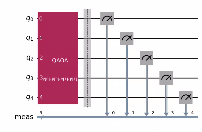
Use QAOAAnsatz to construct the parametrized QAOA circuit from the cost Hamiltonian. Here we use reps=2 (two QAOA layers, four parameters: $\beta_0, \beta_1, \gamma_0, \gamma_1$ ).

circuit = QAOAAnsatz(cost_operator=cost_hamiltonian, reps=2)
circuit.measure_all()

circuit.draw("mpl")

Output:

circuit.parameters

Output:

ParameterView([ParameterVectorElement(β[0]), ParameterVectorElement(β[1]), ParameterVectorElement(γ[0]), ParameterVectorElement(γ[1])])

Step 2: Optimize problem for quantum hardware execution

Transpile the abstract circuit into hardware-native instructions. This step handles qubit mapping, gate decomposition, routing, and error suppression. See the transpilation documentation for more information.

service = QiskitRuntimeService()
backend = service.least_busy(
    operational=True, simulator=False, min_num_qubits=127
)
print(backend)

# Create pass manager for transpilation. Level 3 is the most aggressive
# preset: slower to transpile, but produces shorter circuits that are
# more robust to hardware noise.
pm = generate_preset_pass_manager(optimization_level=3, backend=backend)

candidate_circuit = pm.run(circuit)
candidate_circuit.draw("mpl", fold=False, idle_wires=False)

Output:

<IBMBackend('ibm_pittsburgh')>

Step 3: Execute using Qiskit primitives

The QAOA optimization loop runs inside a Qiskit Runtime session to keep the device reserved across iterations. An Estimator evaluates $\langle H_C \rangle$ at each step, and a classical optimizer (COBYLA) updates the parameters until convergence.

Illustration showing the behavior of Single job, Batch, and Session runtime modes.

Define initial parameters and run the optimization loop:

# QAOA doesn't prescribe principled default angles — any bounded choice
# works as a warm start for problems this small. beta and gamma are
# periodic (beta in [0, pi] and gamma in [0, 2*pi] modulo the underlying
# Pauli-rotation periods), and pi/2 and pi are just midpoints of those
# ranges. For harder problems you would typically warm start from known
# good angles or transfer parameters from smaller instances.
initial_gamma = np.pi
initial_beta = np.pi / 2
init_params = [initial_beta, initial_beta, initial_gamma, initial_gamma]

def cost_func_estimator(params, ansatz, hamiltonian, estimator):
    # transform the observable defined on virtual qubits to
    # an observable defined on all physical qubits
    isa_hamiltonian = hamiltonian.apply_layout(ansatz.layout)

    pub = (ansatz, isa_hamiltonian, params)
    job = estimator.run([pub])

    results = job.result()[0]
    cost = results.data.evs

    objective_func_vals.append(cost)

    return cost

objective_func_vals = []  # Global variable
with Session(backend=backend) as session:
    # If using qiskit-ibm-runtime<0.24.0, change `mode=` to `session=`
    estimator = Estimator(mode=session)
    estimator.options.default_shots = 1000

    # Set simple error suppression/mitigation options
    estimator.options.dynamical_decoupling.enable = True
    estimator.options.dynamical_decoupling.sequence_type = "XY4"
    estimator.options.twirling.enable_gates = True
    estimator.options.twirling.num_randomizations = "auto"
    estimator.options.environment.job_tags = ["TUT_QAOA"]

    result = minimize(
        cost_func_estimator,
        init_params,
        args=(candidate_circuit, cost_hamiltonian, estimator),
        method="COBYLA",
        tol=1e-2,
    )
    print(result)

Output:

 message: Return from COBYLA because the trust region radius reaches its lower bound.
 success: True
  status: 0
     fun: -2.0402211719947774
       x: [ 3.041e+00  1.212e+00  2.081e+00  4.471e+00]
    nfev: 36
   maxcv: 0.0

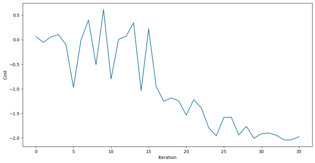
The optimizer was able to reduce the cost and find better parameters for the circuit.

A smoothly decreasing curve that plateaus is the signature of convergence. A noisy, non-monotonic curve usually indicates that something upstream needs attention; common causes are too few shots per evaluation (high estimator variance), poor initial parameters, or a circuit whose depth is dominated by hardware noise. COBYLA is derivative-free and fairly robust to moderate noise, but when the noise swamps the actual cost improvements per step, its linear-approximation model can no longer tell real descent from random jitter and the optimizer wanders.

plt.figure(figsize=(12, 6))
plt.plot(objective_func_vals)
plt.xlabel("Iteration")
plt.ylabel("Cost")
plt.show()

Output:

Assign the optimized parameters and sample the final distribution using the Sampler primitive.

optimized_circuit = candidate_circuit.assign_parameters(result.x)
optimized_circuit.draw("mpl", fold=False, idle_wires=False)

Output:

# If using qiskit-ibm-runtime<0.24.0, change `mode=` to `backend=`
sampler = Sampler(mode=backend)
sampler.options.default_shots = 10000

# Set simple error suppression/mitigation options
sampler.options.dynamical_decoupling.enable = True
sampler.options.dynamical_decoupling.sequence_type = "XY4"
sampler.options.twirling.enable_gates = True
sampler.options.twirling.num_randomizations = "auto"

sampler.options.environment.job_tags = ["TUT_QAOA"]

pub = (optimized_circuit,)
job = sampler.run([pub], shots=int(1e4))
counts_int = job.result()[0].data.meas.get_int_counts()
counts_bin = job.result()[0].data.meas.get_counts()
shots = sum(counts_int.values())
final_distribution_int = {key: val / shots for key, val in counts_int.items()}
final_distribution_bin = {key: val / shots for key, val in counts_bin.items()}
print(final_distribution_int)

Output:

{18: 0.039, 5: 0.0665, 20: 0.0973, 29: 0.0063, 9: 0.0899, 13: 0.0379, 2: 0.0047, 1: 0.0153, 11: 0.0932, 14: 0.0327, 12: 0.0314, 25: 0.0193, 21: 0.0398, 6: 0.0224, 4: 0.0197, 10: 0.0387, 3: 0.0181, 26: 0.07, 17: 0.0327, 19: 0.0332, 22: 0.0914, 24: 0.007, 0: 0.0033, 8: 0.0066, 30: 0.0158, 28: 0.0169, 27: 0.0222, 16: 0.0073, 7: 0.0057, 23: 0.0062, 15: 0.0054, 31: 0.0041}

Step 4: Post-process and return result in desired classical format

Extract the most likely bitstring from the sampled distribution. This represents the best cut found by QAOA.

# auxiliary functions to sample most likely bitstring
def to_bitstring(integer, num_bits):
    result = np.binary_repr(integer, width=num_bits)
    return [int(digit) for digit in result]


keys = list(final_distribution_int.keys())
values = list(final_distribution_int.values())
most_likely = keys[np.argmax(np.abs(values))]
most_likely_bitstring = to_bitstring(most_likely, len(graph))
most_likely_bitstring.reverse()

print("Result bitstring:", most_likely_bitstring)

Output:

Result bitstring: [0, 0, 1, 0, 1]

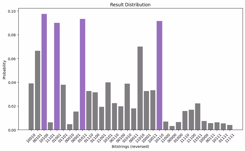
plt.rcParams.update({"font.size": 10})
final_bits = final_distribution_bin
values = np.abs(list(final_bits.values()))
top_4_values = sorted(values, reverse=True)[:4]
positions = []
for value in top_4_values:
    positions.append(np.where(values == value)[0])
fig = plt.figure(figsize=(11, 6))
ax = fig.add_subplot(1, 1, 1)
plt.xticks(rotation=45)
plt.title("Result Distribution")
plt.xlabel("Bitstrings (reversed)")
plt.ylabel("Probability")
ax.bar(list(final_bits.keys()), list(final_bits.values()), color="tab:grey")
for p in positions:
    ax.get_children()[int(p[0])].set_color("tab:purple")
plt.show()

Output:

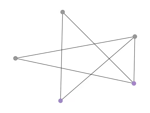
Visualize best cut

From the optimal bitstring, you can then visualize this cut on the original graph.

# auxiliary function to plot graphs
def plot_result(G, x):
    colors = ["tab:grey" if i == 0 else "tab:purple" for i in x]
    pos, _default_axes = rx.spring_layout(G), plt.axes(frameon=True)
    rx.visualization.mpl_draw(
        G, node_color=colors, node_size=100, alpha=0.8, pos=pos
    )


plot_result(graph, most_likely_bitstring)

Output:

Now, calculate the value of the cut:

def evaluate_sample(x: Sequence[int], graph: rx.PyGraph) -> float:
    assert len(x) == len(
        list(graph.nodes())
    ), "The length of x must coincide with the number of nodes in the graph."
    return sum(
        x[u] * (1 - x[v]) + x[v] * (1 - x[u])
        for u, v in list(graph.edge_list())
    )


cut_value = evaluate_sample(most_likely_bitstring, graph)
print("The value of the cut is:", cut_value)

Output:

The value of the cut is: 5

For a graph this small, the true optimum is easy to brute-force, so you can double-check the results by comparing the QAOA result against the exact answer.

# Classical baseline: enumerate all 2**n_small bitstrings and take the best cut.
def brute_force_max_cut(graph: rx.PyGraph) -> tuple[int, list[int]]:
    n = len(list(graph.nodes()))
    best_cut = -1
    best_x: list[int] = []
    for i in range(2**n):
        x = [(i >> k) & 1 for k in range(n)]
        cut = evaluate_sample(x, graph)
        if cut > best_cut:
            best_cut = int(cut)
            best_x = x
    return best_cut, best_x


classical_best, classical_x = brute_force_max_cut(graph)
print(f"Classical optimum (brute force): {classical_best}")
print(f"QAOA cut value:                  {cut_value}")

Output:

Classical optimum (brute force): 5
QAOA cut value:                  5

Large-scale hardware example

You have access to many devices with over 100 qubits on IBM Quantum Platform. Select one on which to solve max-cut on a 100-node weighted graph. This is a "utility-scale" problem. The workflow follows the same steps as above, applied to a much larger graph.

End-to-end workflow at utility scale

All four steps are shown below, applied to the 100-node graph. The structure is the same as the small-scale walkthrough: map, transpile, execute, post-process — but with a larger problem and split across the four cells below for clarity.

# Precomputed parity lookup table: _PARITY[b] = +1 if popcount(b) is even, else -1.
# We use this to vectorize expectation-value evaluation across all Pauli terms.
_PARITY = np.array(
    [-1 if bin(i).count("1") % 2 else 1 for i in range(256)],
    dtype=np.complex128,
)


def evaluate_sparse_pauli(state: int, observable: SparsePauliOp) -> complex:
    """Expectation value of a SparsePauliOp on a single computational-basis state.

    For a Z-only observable (which QAOA cost Hamiltonians are, after the
    QUBO-to-Hamiltonian mapping), the eigenvalue of each Pauli term on a
    computational-basis state is simply (-1)**popcount(z_mask AND state),
    i.e., the parity of the bitwise-AND of the term's Z-support and the
    measured bitstring.

    This routine packs the Z-support of every Pauli term into bytes, ANDs
    them against the measured state in a single vectorized op, and looks up
    the parity in _PARITY. For a 100-qubit / ~hundreds-of-terms Hamiltonian
    over 10_000 samples, this is dramatically faster than calling
    SparsePauliOp.expectation_value per sample.
    """
    packed_uint8 = np.packbits(observable.paulis.z, axis=1, bitorder="little")
    state_bytes = np.frombuffer(
        state.to_bytes(packed_uint8.shape[1], "little"), dtype=np.uint8
    )
    reduced = np.bitwise_xor.reduce(packed_uint8 & state_bytes, axis=1)
    return np.sum(observable.coeffs * _PARITY[reduced])


def best_solution(samples, hamiltonian):
    """Return the sampled bitstring (as int) with the lowest Hamiltonian cost."""
    min_cost = float("inf")
    min_sol = None
    for bit_str in samples.keys():
        candidate_sol = int(bit_str)
        fval = evaluate_sparse_pauli(candidate_sol, hamiltonian).real
        if fval <= min_cost:
            min_cost = fval
            min_sol = candidate_sol
    return min_sol


def _plot_cdf(objective_values: dict, ax, color):
    x_vals = sorted(objective_values.keys(), reverse=True)
    y_vals = np.cumsum([objective_values[x] for x in x_vals])
    ax.plot(x_vals, y_vals, color=color)


def plot_cdf(dist, ax, title):
    _plot_cdf(dist, ax, "C1")
    ax.vlines(min(list(dist.keys())), 0, 1, "C1", linestyle="--")
    ax.set_title(title)
    ax.set_xlabel("Objective function value")
    ax.set_ylabel("Cumulative distribution function")
    ax.grid(alpha=0.3)


def samples_to_objective_values(samples, hamiltonian):
    """Convert the samples to values of the objective function."""
    objective_values = defaultdict(float)
    for bit_str, prob in samples.items():
        candidate_sol = int(bit_str)
        fval = evaluate_sparse_pauli(candidate_sol, hamiltonian).real
        objective_values[fval] += prob
    return objective_values

Step 1: Build the graph, cost Hamiltonian, and ansatz.

# Step 1: build the 100-node graph, cost Hamiltonian, and QAOA ansatz.
n_large = 100
graph_100 = rx.PyGraph()
graph_100.add_nodes_from(np.arange(0, n_large, 1))
elist = []
for edge in backend.coupling_map:
    if edge[0] < n_large and edge[1] < n_large:
        elist.append((edge[0], edge[1], 1.0))
graph_100.add_edges_from(elist)

max_cut_paulis_100 = build_max_cut_paulis(graph_100)
cost_hamiltonian_100 = SparsePauliOp.from_sparse_list(
    max_cut_paulis_100, n_large
)

circuit_100 = QAOAAnsatz(cost_operator=cost_hamiltonian_100, reps=1)
circuit_100.measure_all()

Step 2: Transpile for the selected hardware backend.

# Step 2: transpile for hardware.
pm = generate_preset_pass_manager(optimization_level=3, backend=backend)
candidate_circuit_100 = pm.run(circuit_100)

Step 3: Run the QAOA optimization loop inside a session, then sample.

# Step 3: run the QAOA optimization loop on the device, then sample the
# final distribution with the optimized parameters.
initial_gamma = np.pi
initial_beta = np.pi / 2
init_params = [initial_beta, initial_gamma]

objective_func_vals = []  # Global variable
with Session(backend=backend) as session:
    estimator = Estimator(mode=session)
    estimator.options.default_shots = 1000

    # Set simple error suppression/mitigation options
    estimator.options.dynamical_decoupling.enable = True
    estimator.options.dynamical_decoupling.sequence_type = "XY4"
    estimator.options.twirling.enable_gates = True
    estimator.options.twirling.num_randomizations = "auto"
    estimator.options.environment.job_tags = ["TUT_QAOA"]

    result = minimize(
        cost_func_estimator,
        init_params,
        args=(candidate_circuit_100, cost_hamiltonian_100, estimator),
        method="COBYLA",
    )
    print(result)

# Assign optimal parameters and sample the final distribution.
optimized_circuit_100 = candidate_circuit_100.assign_parameters(result.x)

sampler = Sampler(mode=backend)
sampler.options.default_shots = 10000

# Set simple error suppression/mitigation options
sampler.options.dynamical_decoupling.enable = True
sampler.options.dynamical_decoupling.sequence_type = "XY4"
sampler.options.twirling.enable_gates = True
sampler.options.twirling.num_randomizations = "auto"

# Add a unique tag to the job execution
sampler.options.environment.job_tags = ["TUT_QAOA"]

pub = (optimized_circuit_100,)
job = sampler.run([pub], shots=int(1e4))

counts_int = job.result()[0].data.meas.get_int_counts()
shots = sum(counts_int.values())
final_distribution_100_int = {
    key: val / shots for key, val in counts_int.items()
}

Output:

 message: Return from COBYLA because the trust region radius reaches its lower bound.
 success: True
  status: 0
     fun: -17.172689238986344
       x: [ 2.574e+00  4.166e+00]
    nfev: 28
   maxcv: 0.0

Step 4: Post-process the sampled distribution to extract the best cut.

# Step 4: find the best-cost sample and evaluate its cut value.
best_sol_100 = best_solution(final_distribution_100_int, cost_hamiltonian_100)
best_sol_bitstring_100 = to_bitstring(int(best_sol_100), len(graph_100))
best_sol_bitstring_100.reverse()

print("Result bitstring:", best_sol_bitstring_100)

cut_value_100 = evaluate_sample(best_sol_bitstring_100, graph_100)
print("The value of the cut is:", cut_value_100)

Output:

Result bitstring: [1, 1, 0, 1, 1, 0, 1, 1, 1, 0, 1, 0, 1, 1, 1, 0, 1, 1, 1, 1, 0, 0, 1, 0, 0, 1, 1, 0, 1, 0, 1, 0, 1, 1, 0, 1, 1, 0, 0, 0, 0, 0, 1, 1, 0, 1, 0, 0, 0, 1, 0, 0, 1, 0, 1, 0, 0, 1, 1, 1, 1, 1, 0, 1, 0, 1, 0, 0, 0, 1, 0, 1, 0, 1, 0, 0, 0, 0, 1, 0, 0, 1, 0, 1, 1, 1, 1, 0, 1, 0, 1, 0, 1, 1, 1, 0, 1, 1, 1, 0]
The value of the cut is: 156

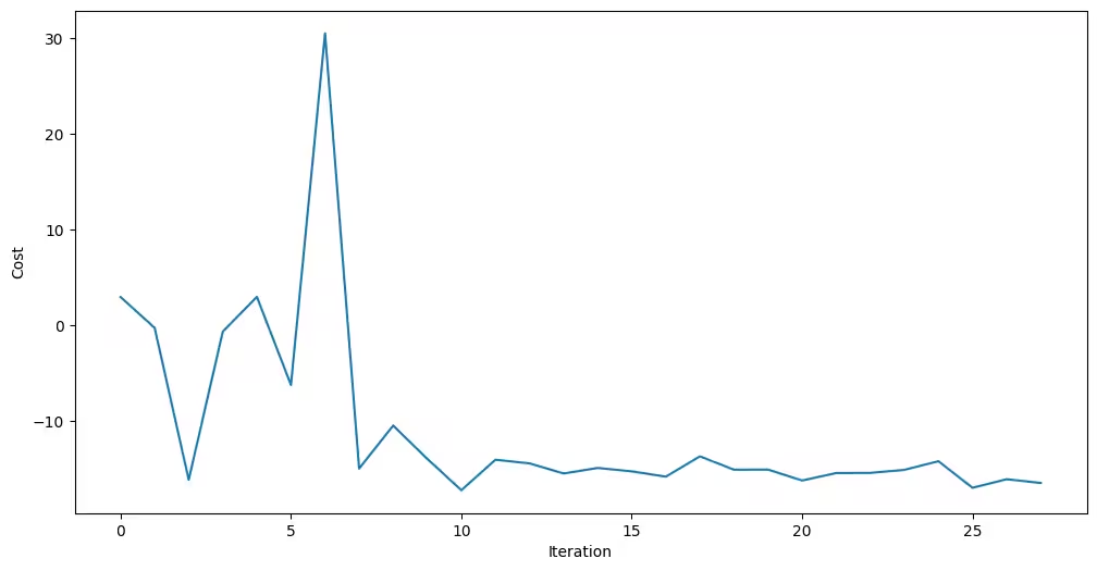
Check that the cost minimized in the optimization loop has converged, and visualize results.

# Plot convergence
plt.figure(figsize=(12, 6))
plt.plot(objective_func_vals)
plt.xlabel("Iteration")
plt.ylabel("Cost")
plt.show()

# Visualize the cut
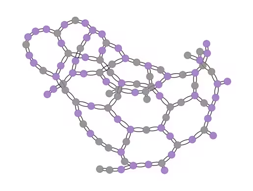
plot_result(graph_100, best_sol_bitstring_100)

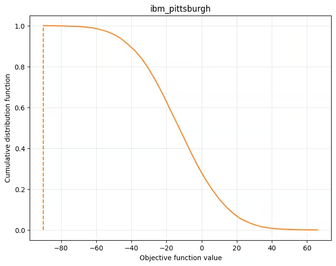
# Plot cumulative distribution function
result_dist = samples_to_objective_values(
    final_distribution_100_int, cost_hamiltonian_100
)
fig, ax = plt.subplots(1, 1, figsize=(8, 6))
plot_cdf(result_dist, ax, backend.name)

Output:

Next steps

If you found this work interesting, you might be interested in the following material:

Recommendations

Advanced techniques for QAOA — explores advanced strategies for improving QAOA performance
Multi-objective optimization challenge — put your skills to the test with this community challenge on multi-objective quantum optimization
Transpilation documentation for fine-tuning circuit optimization
Error suppression and mitigation for improving hardware results