Ground-state energy estimation of the Heisenberg chain with VQE

Usage estimate: 37 minutes on a Heron processor (NOTE: This is an estimate only. Your runtime might vary.)

Background

This tutorial shows how to build, deploy, and run a Qiskit pattern for simulating a Heisenberg chain and estimating its ground state energy using the SPSA optimizer. For more information about Qiskit pattern, refer to the documentation.

Requirements

Before starting this tutorial, ensure that you have the following installed:

Qiskit SDK 2.0 or later, with visualization support (pip install 'qiskit[visualization]')
Qiskit Runtime 0.44 or later (pip install qiskit-ibm-runtime)

Setup

import numpy as np
import matplotlib.pyplot as plt
from typing import Sequence
 
from qiskit import QuantumCircuit
from qiskit.quantum_info import SparsePauliOp
from qiskit.primitives import BaseEstimatorV2
from qiskit.circuit.library import XGate
from qiskit.circuit.library import efficient_su2
from qiskit.transpiler import PassManager
from qiskit.transpiler.preset_passmanagers import generate_preset_pass_manager
from qiskit.transpiler.passes.scheduling import (
    ALAPScheduleAnalysis,
    PadDynamicalDecoupling,
)
from qiskit_ibm_runtime import QiskitRuntimeService, Session, EstimatorV2
 
 
def visualize_results(results):
    plt.plot(results["cost_history"], lw=2)
    plt.xlabel("Number of function evaluations")
    plt.ylabel("Energy")
    plt.show()

Step 1: Map classical inputs to a quantum problem

Input: Number of spins
Output: Ansatz and Hamiltonian modeling the Heisenberg chain

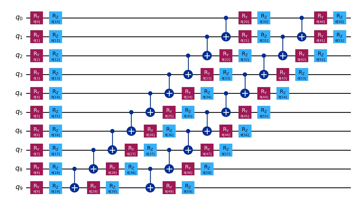
Construct an ansatz and Hamiltonian which model a 10-spin Heisenberg chain. First, we import some generic packages and create a couple of helper functions.

num_spins = 10
ansatz = efficient_su2(num_qubits=num_spins, reps=2)
 
service = QiskitRuntimeService(
    channel="ibm_cloud",
    token=<YOUR_API_TOKEN>  # Replace with your actual API token
    instance = <YOUR_INSTANCE_NAME>  # Replace with your instance name if needed
)
backend = service.least_busy(
    operational=True, min_num_qubits=num_spins, simulator=False
)
 
coupling = backend.target.build_coupling_map()
reduced_coupling = coupling.reduce(list(range(num_spins)))
 
edge_list = reduced_coupling.graph.edge_list()
ham_list = []
 
for edge in edge_list:
    ham_list.append(("ZZ", edge, 0.5))
    ham_list.append(("YY", edge, 0.5))
    ham_list.append(("XX", edge, 0.5))
 
for qubit in reduced_coupling.physical_qubits:
    ham_list.append(("Z", [qubit], np.random.random() * 2 - 1))
 
hamiltonian = SparsePauliOp.from_sparse_list(ham_list, num_qubits=num_spins)
 
ansatz.draw("mpl", style="iqp")

Output:

qiskit_runtime_service._discover_account:WARNING:2026-01-12 07:30:32,269: Loading account with the given token. A saved account will not be used.

<Figure size 1541.66x869.556 with 1 Axes>

Step 2: Optimize problem for quantum hardware execution

Input: Abstract circuit, observable
Output: Target circuit and observable, optimized for the selected QPU

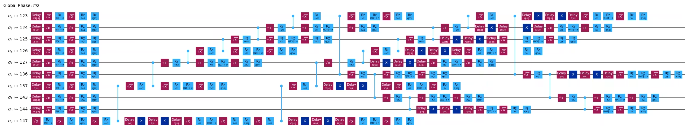
Use the generate_preset_pass_manager function from Qiskit to automatically generate an optimization routine for our circuit with respect to the selected QPU. We choose optimization_level=3, which provides the highest level of optimization of the preset pass managers. We also include ALAPScheduleAnalysis and PadDynamicalDecoupling scheduling passes to suppress decoherence errors.

target = backend.target
pm = generate_preset_pass_manager(optimization_level=3, target=target)
pm.scheduling = PassManager(
    [
        ALAPScheduleAnalysis(durations=target.durations()),
        PadDynamicalDecoupling(
            durations=target.durations(),
            dd_sequence=[XGate(), XGate()],
            pulse_alignment=target.pulse_alignment,
        ),
    ]
)
isa_ansatz = pm.run(ansatz)
isa_observable = hamiltonian.apply_layout(isa_ansatz.layout)
isa_ansatz.draw("mpl", scale=0.6, style="iqp", fold=-1, idle_wires=False)

Output:

<Figure size 2935.1x521.733 with 1 Axes>

Step 3: Execute using Qiskit primitives

Input: Target circuit and observable
Output: Results of optimization

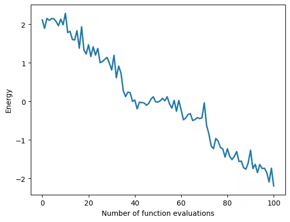
Minimize the estimated ground state energy of the system by optimizing the circuit parameters. Use the Estimator primitive from Qiskit Runtime to evaluate the cost function during optimization.

Since we optimized the circuit for the backend in Step 2, we can avoid doing transpilation on the Runtime server by setting skip_transpilation=True and passing the optimized circuit. For this demo, we will run on a QPU using qiskit-ibm-runtime primitives. To run with qiskit statevector-based primitives, replace the block of code using Qiskit IBM Runtime primitives with the commented block.

In this tutorial we use SPSA, which is a gradient based optimizer. Next we give a brief introduction to it, and provide the code to implement SPSA using Qiskit 2.0.

Introducing SPSA

Simultaneous Perturbation Stochastic Approximation (SPSA) [1] is an optimization algorithm that approximates the entire gradient vector using 2 function calls only at each iteration. Let $f:\mathbb{R}^p\rightarrow \mathbb{R}$ be the cost function with $p$ parameters to be optimized, and $x_i\in \mathbb{R}^p$ be the parameter vector at the $i$ -th step of iteration. To compute the gradient, a random vector $\Delta_i$ of size $p$ is created, where each element $\Delta_{ij}$ , $\forall$ $j\in \{1,2,...,p\}$ , is uniformly sampled from $\{-1, 1\}$ . Next, each element of the random vector $\Delta_i$ is multiplied with a small value $c_i$ to create a random perturbation. The gradient is then estimated as

$[\nabla f(x_i)]_j \approx \frac{f(x_i + c_i \Delta_i) - f(x_i - c_i \Delta_i)}{2c_i\Delta_{ij}}.$

Intuitively, since a random perturbation is applied during the gradient estimation, it is expectation that small deviations in the exact values of $f$ coming from noise can be tolerated and accounted for. In fact, SPSA is particularly known to be robust against noise, and requires only two hardware calls for each iteration. It is, therefore, one of the highly preferred optimizers for implementing variational algorithms.

In this tutorial, the hyperparameters for the $i$ -th iteration, $a_i$ and $c_i$ , are computed as $a_i = a/(A + i + 1)^\alpha$ and $c_i = c / (i+1)^\gamma$ , where the constant values are taken as $A = 30$ , $\alpha = 0.9$ , $a = 0.3$ , $c = 0.1$ , and $\gamma = 0.4$ . These values are selected from [2]. Appropriate tuning of hyperparameters is necessary for extracting a good performance out of SPSA.

def spsa(
        fun, x0, args=(),
        A = 30, alpha = 0.9, a = 0.3, c = 0.1, gamma = 0.4, maxiter=100
    ):
    nparams = len(x0)
    x = np.copy(x0)
    
    for i in range(maxiter):
        a_i = a / (A + i + 1) ** alpha
        c_i = c / (i + 1) ** gamma
        delta_i = np.random.choice([-1, 1], nparams)
 
        # two hardware calls
        eval_1 = fun(x + c_i * delta_i, *args)
        eval_2 = fun(x - c_i * delta_i, *args)
 
        # compute the gradient and update the parameters
        grad = (eval_1 - eval_2) / (2 * c_i) * np.reciprocal(delta_i)
        x = x - a_i * grad
 
    return x

def cost_func(
    params: Sequence,
    ansatz: QuantumCircuit,
    hamiltonian: SparsePauliOp,
    estimator: BaseEstimatorV2,
    cost_history_dict: dict,
) -> float:
    """Ground state energy evaluation."""
    energy = estimator.run([(ansatz, hamiltonian, [params])]).result()[0].data.evs
 
    cost_history_dict['iters'] += 1
    cost_history_dict['prev_vector'] = list(params)
    cost_history_dict['cost_history'].append(float(energy[0]))
 
    print(
        f"Fx Iters. done: {cost_history_dict['iters']} [Current cost: {round(energy[0], 5)}]",
        end="\r",
    )
    
    return energy
 
 
def solve(x0, isa_ansatz, isa_observable, maxiter=150):
    cost_history_dict = {
        "prev_vector": None,
        "iters": 0,
        "cost_history": [],
        'y_min': None,
    }
 
    # Evaluate the problem using a QPU via Qiskit IBM Runtime
    with Session(backend=backend) as session:
        estimator = EstimatorV2()
        estimator.skip_transpilation = True
        x_opt = spsa(
            cost_func,
            x0=x0,
            args=(isa_ansatz, isa_observable, estimator, cost_history_dict),
            maxiter=maxiter
        )
 
        y_min = cost_func(x_opt, isa_ansatz, isa_observable, estimator, cost_history_dict)
        
    return y_min, cost_history_dict

np.random.seed(42)
num_params = ansatz.num_parameters
params = 2 * np.pi * np.random.random(num_params)

Here we set the maxiter = 50. Note that since each iteration requires two calls to the function to compute gradient, the total number of function calls will be $2 \times \text{maxiter}$ . The maxiter can be increased to any higher value for better energy estimation.

maxiter = 50
spsa_min, spsa_history = solve(params, isa_ansatz, isa_observable, maxiter=maxiter)

Output:

Fx Iters. done: 101 [Current cost: -2.19621]

Step 4: Post-process and return result in desired classical format

Input: Ground state energy estimates during optimization
Output: Estimated ground state energy

print(f'Estimated ground state energy: {spsa_min}')

Output:

Estimated ground state energy: [-2.19621239]

results = {
    'spsa': spsa_history,
}
 
visualize_results(spsa_history)

Output:

<Figure size 640x480 with 1 Axes>

References

[1] Spall, J. C. (2002). Implementation of the simultaneous perturbation algorithm for stochastic optimization. IEEE Transactions on Aerospace and Electronic Systems, 34(3), 817-823.

[2] Sahin, M. Emre, et al (2025). Qiskit Machine Learning: an open-source library for quantum machine learning tasks at scale on quantum hardware and classical simulators. arXiv:2505.17756.

Tutorial survey

Please take this short survey to provide feedback on this tutorial. Your insights will help us improve our content offerings and user experience.

Link to survey