Simulation of kicked Ising Hamiltonian with dynamic circuits

Usage estimate: 7.5 minutes on a Heron r3 processor. (NOTE: This is an estimate only. Your runtime may vary.)

Dynamic circuits are circuits with classical feedforward - in other words, they are mid-circuit measurements followed by classical logic operations that determine quantum operations conditioned on the classical output. In this tutorial, we simulate the kicked Ising model on a hexagonal lattice of spins and use dynamic circuits to realize interactions beyond the physical connectivity of the hardware.

The Ising model has been studied extensively across areas of physics. It models spins that undergo Ising interactions between lattice sites, as well as kicks from the local magnetic field on each site. The Trotterized time evolution of the spins considered in this tutorial, taken from [1], is given by the following unitary:

U(\theta)=\left(\prod_{\langle j, k\rangle} \exp \left(i \frac{\pi}{8} Z_j Z_k\right)\right)\left(\prod_j \exp \left(-i \frac{\theta}{2} X_j\right)\right)

To probe the spin dynamics, we study the average magnetization of the spins at each site as a function of Trotter steps. Hence, we construct the following observable:

\langle O\rangle = \frac{1}{N} \sum_i \langle Z_i \rangle

To realize the ZZ interaction between lattice sites, we present a solution using the dynamic circuit feature, leading to a significantly shorter two-qubit depth compared to the standard routing method with SWAP gates. On the other hand, the classical feedforward operations in dynamic circuits typically have longer execution times than quantum gates; hence, dynamic circuits have limitations and tradeoffs. We also present a way to add a dynamical decoupling sequence on idling qubits during the classical feedforward operation using the stretch duration.

Requirements

Before starting this tutorial, ensure that you have the following installed:

Qiskit SDK v2.0 or later with visualization support
Qiskit Runtime v0.37 or later with visualization support (pip install 'qiskit-ibm-runtime[visualization]')
Rustworkx graph library (pip install rustworkx)
Qiskit Aer (pip install qiskit-aer)

Set up

import numpy as np
from typing import List
import rustworkx as rx
import matplotlib.pyplot as plt
from rustworkx.visualization import mpl_draw
from qiskit.circuit import (
    Parameter,
    QuantumCircuit,
    QuantumRegister,
    ClassicalRegister,
)
from qiskit.transpiler import CouplingMap
from qiskit.quantum_info import SparsePauliOp
from qiskit.circuit.classical import expr
from qiskit.transpiler.preset_passmanagers import (
    generate_preset_pass_manager,
)
from qiskit.transpiler import PassManager
from qiskit.circuit.library import RZGate, XGate
from qiskit.transpiler.passes import (
    ALAPScheduleAnalysis,
    PadDynamicalDecoupling,
)
 
from qiskit.transpiler.basepasses import TransformationPass
from qiskit.circuit.measure import Measure
from qiskit.transpiler.passes.utils.remove_final_measurements import (
    calc_final_ops,
)
from qiskit.circuit import Instruction
 
from qiskit.visualization import plot_circuit_layout
from qiskit.circuit.tools import pi_check
 
from qiskit_aer import AerSimulator
from qiskit_aer.primitives import SamplerV2 as Aer_Sampler
 
from qiskit_ibm_runtime import (
    QiskitRuntimeService,
    Batch,
    SamplerV2 as Sampler,
)
from qiskit_ibm_runtime.exceptions import QiskitBackendNotFoundError
from qiskit_ibm_runtime.visualization import (
    draw_circuit_schedule_timing,
)

Step 1: Map classical inputs to a quantum circuit

We start by defining the lattice to simulate. We choose to work with the honeycomb (also called hexagonal) lattice, which is a planar graph with nodes of degree 3. Here, we specify the size of the lattice, the relevant circuit parameters of interest in the Trotterized dynamics. We simulate the Trotterized time evolution under the Ising model under three different $\theta$ values of the local magnetic field.

hex_rows = 3  # specify lattice size
hex_cols = 5
depths = range(9)  # specify Trotter steps
zz_angle = np.pi / 8  # parameter for ZZ interaction
max_angle = np.pi / 2  # max theta angle
points = 3  # number of theta parameters
 
θ = Parameter("θ")
params = np.linspace(0, max_angle, points)

def make_hex_lattice(hex_rows=1, hex_cols=1):
    """Define hexagon lattice."""
    hex_cmap = CouplingMap.from_hexagonal_lattice(
        hex_rows, hex_cols, bidirectional=False
    )
    data = list(hex_cmap.physical_qubits)
    graph = hex_cmap.graph.to_undirected(multigraph=False)
    edge_colors = rx.graph_misra_gries_edge_color(graph)
    layer_edges = {color: [] for color in edge_colors.values()}
    for edge_index, color in edge_colors.items():
        layer_edges[color].append(graph.edge_list()[edge_index])
    return data, layer_edges, hex_cmap, graph

Let's start with a small test example:

hex_rows_test = 1
hex_cols_test = 2
 
data_test, layer_edges_test, hex_cmap_test, graph_test = make_hex_lattice(
    hex_rows=hex_rows_test, hex_cols=hex_cols_test
)
 
# display a small example for illustration
node_colors_test = ["lightblue"] * len(graph_test.node_indices())
pos = rx.graph_spring_layout(
    graph_test,
    k=5 / np.sqrt(len(graph_test.nodes())),
    repulsive_exponent=1,
    num_iter=150,
)
mpl_draw(graph_test, node_color=node_colors_test, pos=pos)

Output:

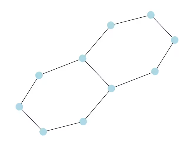
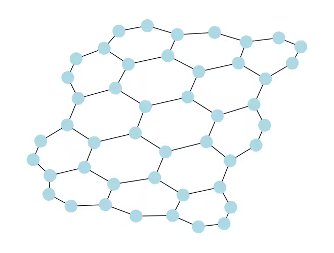
We will use the small example for illustration and simulation. Below we also construct a large example to show the workflow can be extended to large sizes.

data, layer_edges, hex_cmap, graph = make_hex_lattice(
    hex_rows=hex_rows, hex_cols=hex_cols
)
num_qubits = len(data)
print(f"num_qubits = {num_qubits}")
 
# display the honeycomb lattice to simulate
node_colors = ["lightblue"] * len(graph.node_indices())
pos = rx.graph_spring_layout(
    graph,
    k=5 / np.sqrt(num_qubits),
    repulsive_exponent=1,
    num_iter=150,
)
mpl_draw(graph, node_color=node_colors, pos=pos)
plt.show()

Output:

num_qubits = 46

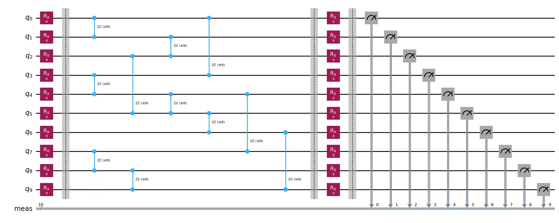
Build unitary circuits

With the problem size and parameters specified, we are now ready to build the parametrized circuit that simulates the Trotterized time evolution of $U(\theta)$ with different Trotter steps, specified by the depth argument. The circuit we construct has alternating layers of Rx( $\theta$ ) gates and Rzz gates. The Rzz gates realize the ZZ interactions between coupled spins, which will be placed between each lattice site specified by the layer_edges argument.

def gen_hex_unitary(
    num_qubits=6,
    zz_angle=np.pi / 8,
    layer_edges=[
        [(0, 1), (2, 3), (4, 5)],
        [(1, 2), (3, 4), (5, 0)],
    ],
    θ=Parameter("θ"),
    depth=1,
    measure=False,
    final_rot=True,
):
    """Build unitary circuit."""
    circuit = QuantumCircuit(num_qubits)
    # Build trotter layers
    for _ in range(depth):
        for i in range(num_qubits):
            circuit.rx(θ, i)
        circuit.barrier()
        for coloring in layer_edges.keys():
            for e in layer_edges[coloring]:
                circuit.rzz(zz_angle, e[0], e[1])
        circuit.barrier()
    # Optional final rotation, set True to be consistent with Ref. [1]
    if final_rot:
        for i in range(num_qubits):
            circuit.rx(θ, i)
    if measure:
        circuit.measure_all()
 
    return circuit

Visualize the small test circuit:

circ_unitary_test = gen_hex_unitary(
    num_qubits=len(data_test),
    layer_edges=layer_edges_test,
    θ=Parameter("θ"),
    depth=1,
    measure=True,
)
circ_unitary_test.draw(output="mpl", fold=-1)

Output:

Similarly, construct the unitary circuits of the large example at different Trotter steps and the observable to estimate the expectation value.

circuits_unitary = []
for depth in depths:
    circ = gen_hex_unitary(
        num_qubits=num_qubits,
        layer_edges=layer_edges,
        θ=Parameter("θ"),
        depth=depth,
        measure=True,
    )
    circuits_unitary.append(circ)

observables_unitary = SparsePauliOp.from_sparse_list(
    [("Z", [i], 1 / num_qubits) for i in range(num_qubits)],
    num_qubits=num_qubits,
)

Build dynamic circuit implementation

This section demonstrates the main dynamic circuit implementation to simulate the same Trotterized time evolution. Note that the honeycomb lattice we want to simulate does not match the heavy lattice of the hardware qubits. One straightforward way to map the circuit to the hardware is to introduce a series of SWAP operations to bring interacting qubits next to each other, to realize the ZZ interaction. Here we highlight an alternative approach using dynamic circuits as a solution, which illustrates that we can use the combination of quantum and real-time classical computation within a circuit in Qiskit to realize interactions beyond nearest-neighbor.

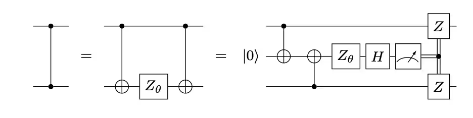
In the dynamic circuit implementation, the ZZ interaction is effectively implemented by using ancilla qubits, mid-circuit measurement, and feedforward. To understand this, note that the ZZ rotations apply a phase factor $e^{i\theta}$ to the state based on its parity. For two qubits, the computational basis states are $|00\rangle$ , $|01\rangle$ , $|10\rangle$ , and $|11\rangle$ . The ZZ rotation gate applies a phase factor to states $|01\rangle$ and $|10\rangle$ whose parity (the number of ones in the state) is odd and leaves even-parity states unchanged. The following describes how we can effectively implement ZZ interactions on two qubits using dynamic circuits.

Compute parity into an ancilla qubit: instead of directly applying ZZ to two qubits, we introduce a third qubit, the ancilla qubit, to store the parity information of the two data qubits. We entangle the ancilla with each data qubit using CX gates from the data qubit to the ancilla qubit.
Apply a single-qubit Z rotation to the ancilla qubit: this is because the ancilla has the parity information of the two data qubits, which effectively implements the ZZ rotation on the data qubits.
Measure the ancilla qubit in the X basis: this is the key step that collapses the state of the ancilla qubit, and the measurement outcome tells us what has happened:
- Measure 0: when a 0 outcome is observed, we have in fact correctly applied a $ZZ(\theta)$ rotation to our data qubits.
- Measure 1: when a 1 outcome is observed, We've applied $ZZ(\theta + \pi)$ instead.
Apply correction gate when measuring 1: If we measured 1, we apply Z gates to the data qubits to "fix" the extra $\pi$ phase.

The resulting circuit is the following:

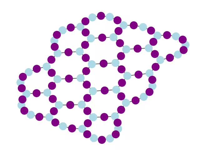
When we adopt this approach to simulate a honeycomb lattice, the resulting circuit embeds perfectly into the hardware with a heavy-hex lattice: all data qubits reside on the degree-3 sites of the lattice, which forms a hexagonal lattice. Every pair of data qubits shares an ancilla qubit residing on a degree-2 site. Below, we construct the qubit lattice for the dynamic circuit implementation, introducing ancilla qubits (shown in the darker purple circles).

def make_lattice(hex_rows=1, hex_cols=1):
    """Define heavy-hex lattice and corresponding lists of data and ancilla nodes."""
    hex_cmap = CouplingMap.from_hexagonal_lattice(
        hex_rows, hex_cols, bidirectional=False
    )
    data = list(hex_cmap.physical_qubits)
 
    heavyhex_cmap = CouplingMap()
    for d in data:
        heavyhex_cmap.add_physical_qubit(d)
 
    # make coupling map
    a = len(data)
    for edge in hex_cmap.get_edges():
        heavyhex_cmap.add_physical_qubit(a)
        heavyhex_cmap.add_edge(edge[0], a)
        heavyhex_cmap.add_edge(edge[1], a)
        a += 1
    ancilla = list(range(len(data), a))
    qubits = data + ancilla
 
    # color edges
    graph = heavyhex_cmap.graph.to_undirected(multigraph=False)
    edge_colors = rx.graph_misra_gries_edge_color(graph)
    layer_edges = {color: [] for color in edge_colors.values()}
    for edge_index, color in edge_colors.items():
        layer_edges[color].append(graph.edge_list()[edge_index])
 
    # construct observable
    obs_hex = SparsePauliOp.from_sparse_list(
        [("Z", [i], 1 / len(data)) for i in data],
        num_qubits=len(qubits),
    )
 
    return (data, qubits, ancilla, layer_edges, heavyhex_cmap, graph, obs_hex)

Visualize the heavy-hex lattice for data qubits and ancilla qubits at a small scale:

(data, qubits, ancilla, layer_edges, heavyhex_cmap, graph, obs_hex) = (
    make_lattice(hex_rows=hex_rows, hex_cols=hex_cols)
)
 
print(f"number of data qubits = {len(data)}")
print(f"number of ancilla qubits = {len(ancilla)}")
 
node_colors = []
for node in graph.node_indices():
    if node in ancilla:
        node_colors.append("purple")
    else:
        node_colors.append("lightblue")
 
pos = rx.graph_spring_layout(
    graph,
    k=1 / np.sqrt(len(qubits)),
    repulsive_exponent=2,
    num_iter=200,
)
 
# Visualize the graph, blue circles are data qubits and purple circles are ancillas
mpl_draw(graph, node_color=node_colors, pos=pos)
plt.show()

Output:

number of data qubits = 46
number of ancilla qubits = 60

Below, we construct the dynamic circuit for the Trotterized time evolution. The RZZ gates are replaced with the dynamic circuit implementation using the steps described above.

def gen_hex_dynamic(
    depth=1,
    zz_angle=np.pi / 8,
    θ=Parameter("θ"),
    hex_rows=1,
    hex_cols=1,
    measure=False,
    add_dd=True,
):
    """Build dynamic circuits."""
    (data, qubits, ancilla, layer_edges, heavyhex_cmap, graph, obs_hex) = (
        make_lattice(hex_rows=hex_rows, hex_cols=hex_cols)
    )
    # Initialize circuit
    qr = QuantumRegister(len(qubits), "qr")
    cr = ClassicalRegister(len(ancilla), "cr")
    circuit = QuantumCircuit(qr, cr)
 
    for k in range(depth):
        # Single-qubit Rx layer
        for d in data:
            circuit.rx(θ, d)
        circuit.barrier()
 
        # CX gates from data qubits to ancilla qubits
        for same_color_edges in layer_edges.values():
            for e in same_color_edges:
                circuit.cx(e[0], e[1])
        circuit.barrier()
 
        # Apply Rz rotation on ancilla qubits and rotate into X basis
        for a in ancilla:
            circuit.rz(zz_angle, a)
            circuit.h(a)
        # Add barrier to align terminal measurement
        circuit.barrier()
 
        # Measure ancilla qubits
        for i, a in enumerate(ancilla):
            circuit.measure(a, i)
        d2ros = {}
        a2ro = {}
        # Retrieve ancilla measurement outcomes
        for a in ancilla:
            a2ro[a] = cr[ancilla.index(a)]
 
        # For each data qubit, retrieve measurement outcomes of neighboring ancilla qubits
        for d in data:
            ros = [a2ro[a] for a in heavyhex_cmap.neighbors(d)]
            d2ros[d] = ros
 
        # Build classical feedforward operations (optionally add DD on idling data qubits)
        for d in data:
            if add_dd:
                circuit = add_stretch_dd(circuit, d, f"data_{d}_depth_{k}")
 
            # # XOR the neighboring readouts of the data qubit; if True, apply Z to it
            ros = d2ros[d]
            parity = ros[0]
            for ro in ros[1:]:
                parity = expr.bit_xor(parity, ro)
            with circuit.if_test(expr.equal(parity, True)):
                circuit.z(d)
 
        # Reset the ancilla if its readout is 1
        for a in ancilla:
            with circuit.if_test(expr.equal(a2ro[a], True)):
                circuit.x(a)
        circuit.barrier()
 
    # Final single-qubit Rx layer to match the unitary circuits
    for d in data:
        circuit.rx(θ, d)
 
    if measure:
        circuit.measure_all()
    return circuit, obs_hex
 
 
def add_stretch_dd(qc, q, name):
    """Add XpXm DD sequence."""
    s = qc.add_stretch(name)
    qc.delay(s, q)
    qc.x(q)
    qc.delay(s, q)
    qc.delay(s, q)
    qc.rz(np.pi, q)
    qc.x(q)
    qc.rz(-np.pi, q)
    qc.delay(s, q)
    return qc

Dynamical decoupling (DD) and support for `stretch` duration

One caveat of using the dynamic circuit implementation to realize the ZZ interaction is that the mid-circuit measurement and the classical feedforward operations typically take a longer time to execute than quantum gates. To suppress qubit decoherence during the idling time for the classical operations to happen, we added a dynamical decoupling (DD) sequence after the measurement operation on the ancilla qubits, and before the conditional Z operation on the data qubit, before the if_test statement.

The DD sequence is added by the function add_stretch_dd(), which uses the stretch durations to determine the time intervals between the DD gates. A stretch duration is a way to specify a stretchable time duration for the delay operation such that the delay duration can grow to fill up the qubit idling time. The duration variables specified by stretch are resolved at compile time into desired durations that satisfy a certain constraint. This is very useful when the timing of DD sequences is essential to achieve good error suppression performance. For more details on the stretch type, see the OpenQASM documentation. Currently, support for the stretch type in Qiskit Runtime is experimental. For details on its usage constraints, please refer to the limitations section of the stretch documentation.

Using the functions defined above, we build the Trotterized time evolution circuits, with and without DD, and the corresponding observables.

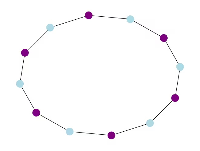
We start by visualizing the dynamic circuit of a small example:

hex_rows_test = 1
hex_cols_test = 1
 
(
    data_test,
    qubits_test,
    ancilla_test,
    layer_edges_test,
    heavyhex_cmap_test,
    graph_test,
    obs_hex_test,
) = make_lattice(hex_rows=hex_rows_test, hex_cols=hex_cols_test)
 
node_colors = []
for node in graph_test.node_indices():
    if node in ancilla_test:
        node_colors.append("purple")
    else:
        node_colors.append("lightblue")
pos = rx.graph_spring_layout(
    graph_test,
    k=5 / np.sqrt(len(qubits_test)),
    repulsive_exponent=2,
    num_iter=150,
)
 
# display a small example for illustration
node_colors_test = ["lightblue"] * len(graph_test.node_indices())
mpl_draw(graph_test, node_color=node_colors, pos=pos)

Output:

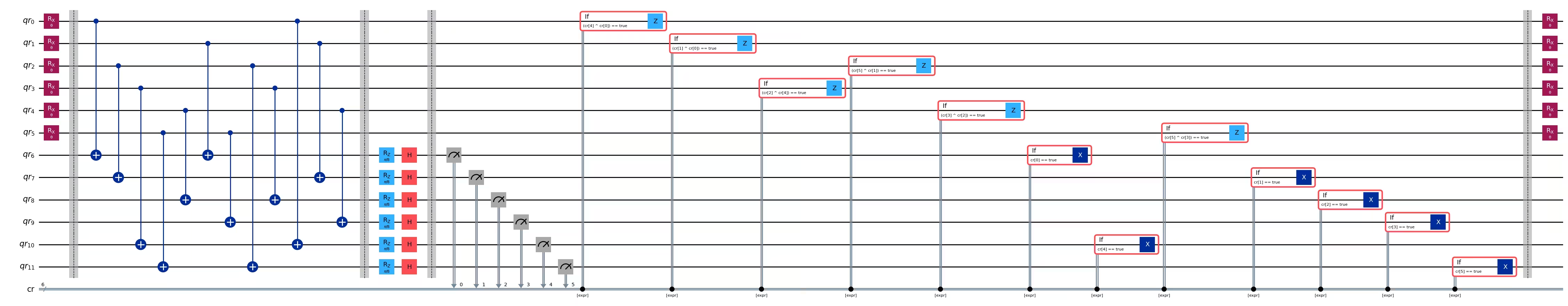
circuit_dynamic_test, obs_dynamic_test = gen_hex_dynamic(
    depth=1,
    θ=Parameter("θ"),
    hex_rows=hex_rows_test,
    hex_cols=hex_cols_test,
    measure=False,
    add_dd=False,
)
circuit_dynamic_test.draw("mpl", fold=-1)

Output:

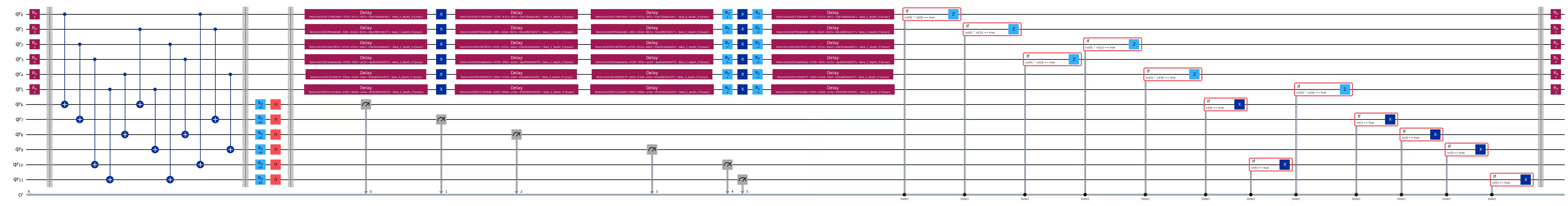
circuit_dynamic_dd_test, _ = gen_hex_dynamic(
    depth=1,
    θ=Parameter("θ"),
    hex_rows=hex_rows_test,
    hex_cols=hex_cols_test,
    measure=False,
    add_dd=True,
)
circuit_dynamic_dd_test.draw("mpl", fold=-1)

Output:

Similarly, construct the dynamic circuits for the large example:

circuits_dynamic = []
circuits_dynamic_dd = []
observables_dynamic = []
for depth in depths:
    circuit, obs = gen_hex_dynamic(
        depth=depth,
        θ=Parameter("θ"),
        hex_rows=hex_rows,
        hex_cols=hex_cols,
        measure=True,
        add_dd=False,
    )
    circuits_dynamic.append(circuit)
 
    circuit_dd, _ = gen_hex_dynamic(
        depth=depth,
        θ=Parameter("θ"),
        hex_rows=hex_rows,
        hex_cols=hex_cols,
        measure=True,
        add_dd=True,
    )
    circuits_dynamic_dd.append(circuit_dd)
    observables_dynamic.append(obs)

Step 2: Optimize problem for hardware execution

We are now ready to transpile the circuit to the hardware. We will transpile both the unitary standard implementation and the dynamic circuit implementation to the hardware.

To transpile to hardware, we first instantiate the backend. If available, we will choose a backend where the MidCircuitMeasure (measure_2) instruction is supported.

service = QiskitRuntimeService()
try:
    backend = service.least_busy(
        operational=True,
        simulator=False,
        use_fractional_gates=True,
        filters=lambda b: "measure_2" in b.supported_instructions,
    )
except QiskitBackendNotFoundError:
    backend = service.least_busy(
        operational=True,
        simulator=False,
        use_fractional_gates=True,
    )

Transpilation for dynamic circuits

First, we transpile the dynamic circuits, with and without adding the DD sequence. To ensure we use the same set of physical qubits in all circuits for more consistent results, we first transpile the circuit once, and then use its layout for all subsequent circuits, specified by initial_layout in the pass manager. We then construct the primitive unified blocs (PUBs) as the Sampler primitive input.

pm_temp = generate_preset_pass_manager(
    optimization_level=3,
    backend=backend,
)
isa_temp = pm_temp.run(circuits_dynamic[-1])
dynamic_layout = isa_temp.layout.initial_index_layout(filter_ancillas=True)
 
pm = generate_preset_pass_manager(
    optimization_level=3, backend=backend, initial_layout=dynamic_layout
)
 
dynamic_isa_circuits = [pm.run(circ) for circ in circuits_dynamic]
dynamic_pubs = [(circ, params) for circ in dynamic_isa_circuits]
 
dynamic_isa_circuits_dd = [pm.run(circ) for circ in circuits_dynamic_dd]
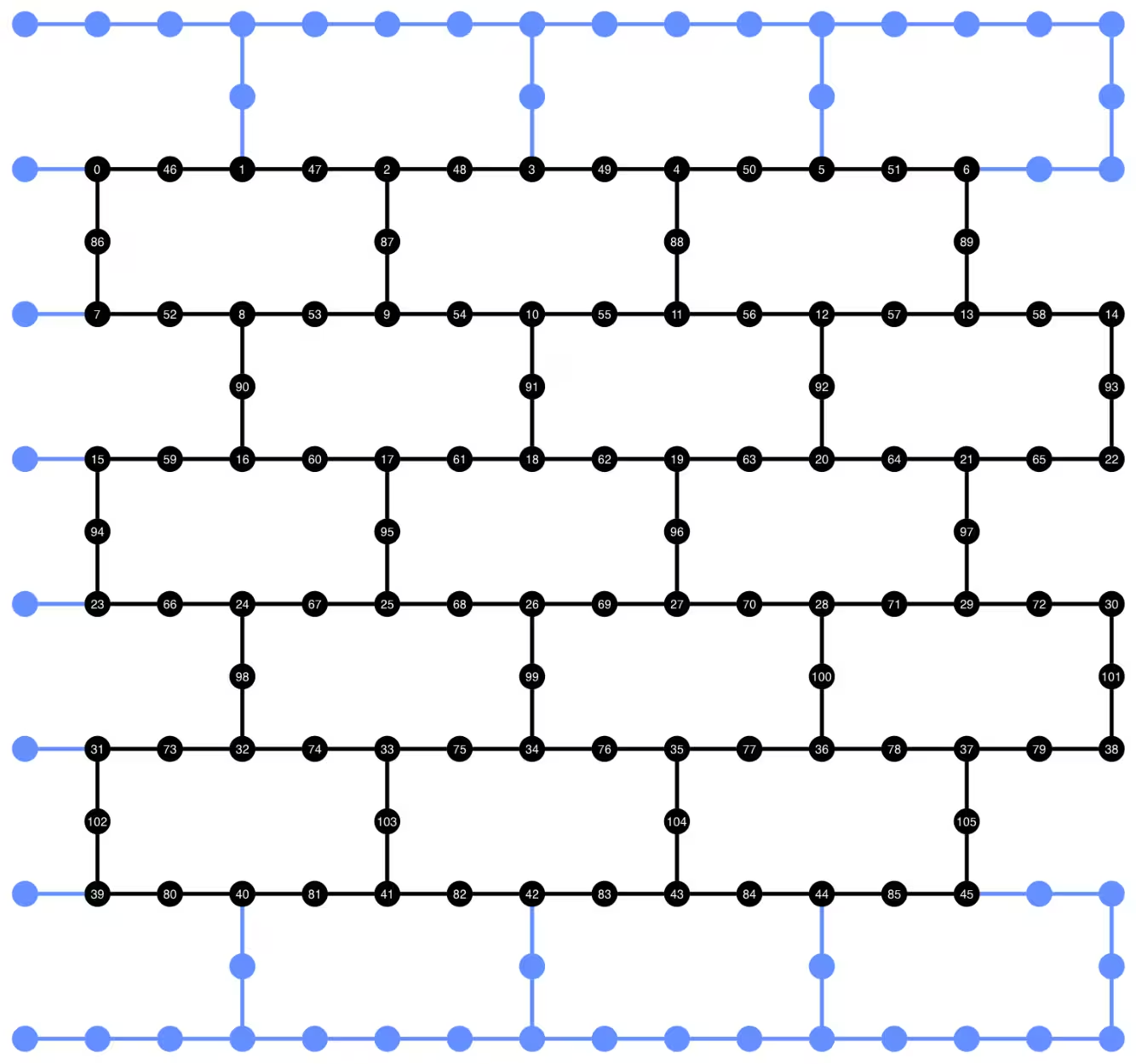
dynamic_pubs_dd = [(circ, params) for circ in dynamic_isa_circuits_dd]

We can visualize the qubit layout of the transpiled circuit below. The black circles show the data qubits and the ancilla qubits used in the dynamic circuit implementation.

def _heron_coords_r2():
    cord_map = np.array(
        [
            [
                0,
                1,
                2,
                3,
                4,
                5,
                6,
                7,
                8,
                9,
                10,
                11,
                12,
                13,
                14,
                15,
                3,
                7,
                11,
                15,
                0,
                1,
                2,
                3,
                4,
                5,
                6,
                7,
                8,
                9,
                10,
                11,
                12,
                13,
                14,
                15,
                1,
                5,
                9,
                13,
                0,
                1,
                2,
                3,
                4,
                5,
                6,
                7,
                8,
                9,
                10,
                11,
                12,
                13,
                14,
                15,
                3,
                7,
                11,
                15,
                0,
                1,
                2,
                3,
                4,
                5,
                6,
                7,
                8,
                9,
                10,
                11,
                12,
                13,
                14,
                15,
                1,
                5,
                9,
                13,
                0,
                1,
                2,
                3,
                4,
                5,
                6,
                7,
                8,
                9,
                10,
                11,
                12,
                13,
                14,
                15,
                3,
                7,
                11,
                15,
                0,
                1,
                2,
                3,
                4,
                5,
                6,
                7,
                8,
                9,
                10,
                11,
                12,
                13,
                14,
                15,
                1,
                5,
                9,
                13,
                0,
                1,
                2,
                3,
                4,
                5,
                6,
                7,
                8,
                9,
                10,
                11,
                12,
                13,
                14,
                15,
                3,
                7,
                11,
                15,
                0,
                1,
                2,
                3,
                4,
                5,
                6,
                7,
                8,
                9,
                10,
                11,
                12,
                13,
                14,
                15,
            ],
            -1
            * np.array([j for i in range(15) for j in [i] * [16, 4][i % 2]]),
        ],
        dtype=int,
    )
 
    hcords = []
    ycords = cord_map[0]
    xcords = cord_map[1]
    for i in range(156):
        hcords.append([xcords[i] + 1, np.abs(ycords[i]) + 1])
 
    return hcords

plot_circuit_layout(
    dynamic_isa_circuits_dd[8],
    backend,
    qubit_coordinates=_heron_coords_r2(),
    view="virtual",
)

Output:

Note

If you get errors about neato not found from plot_circuit_layout(), make sure you have the graphviz package installed and available in your PATH. If it installs into a non-default location (for example, using homebrew on MacOS), you may need to update your PATH environment variable. This can be done inside this notebook using the following:

import os
os.environ['PATH'] = f"path/to/neato{os.pathsep}{os.environ['PATH']}"

dynamic_isa_circuits[1].draw(fold=-1, output="mpl", idle_wires=False)

Output:

dynamic_isa_circuits_dd[1].draw(fold=-1, output="mpl", idle_wires=False)

Output:

Transpile using `MidCircuitMeasure`

MidCircuitMeasure is an addition to the available measurement operations, calibrated specifically to perform mid-circuit measurements. The MidCircuitMeasure instruction maps to the measure_2 instruction supported by the backends. Note that measure_2 is not supported on all backends. You can use service.backends(filters=lambda b: "measure_2" in b.supported_instructions) to find backends that support it. Here, we show how to transpile the circuit so that the mid-circuit measurements defined in the circuit are executed using the MidCircuitMeasure operation, if the backend supports it.

Below, we print the duration for the measure_2 instruction and the standard measure instruction.

print(
    f'Mid-circuit measurement `measure_2` duration: {backend.instruction_durations.get('measure_2',0) * backend.dt * 1e9/1e3} μs'
)
print(
    f'Terminal measurement `measure` duration: {backend.instruction_durations.get('measure',0) * backend.dt *1e9/1e3} μs'
)

Output:

Mid-circuit measurement `measure_2` duration:  1.624 μs
Terminal measurement `measure` duration: 2.2 μs

"""Pass that replaces terminal measures in the middle of the circuit with
MidCircuitMeasure instructions."""
 
 
class ConvertToMidCircuitMeasure(TransformationPass):
    """This pass replaces terminal measures in the middle of the circuit with
    MidCircuitMeasure instructions.
    """
 
    def __init__(self, target):
        super().__init__()
        self.target = target
 
    def run(self, dag):
        """Run the pass on a dag."""
        mid_circ_measure = None
        for inst in self.target.instructions:
            if isinstance(inst[0], Instruction) and inst[0].name.startswith(
                "measure_"
            ):
                mid_circ_measure = inst[0]
                break
        if not mid_circ_measure:
            return dag
 
        final_measure_nodes = calc_final_ops(dag, {"measure"})
        for node in dag.op_nodes(Measure):
            if node not in final_measure_nodes:
                dag.substitute_node(node, mid_circ_measure, inplace=True)
 
        return dag
 
 
pm = PassManager(ConvertToMidCircuitMeasure(backend.target))
 
dynamic_isa_circuits_meas2 = [pm.run(circ) for circ in dynamic_isa_circuits]
dynamic_pubs_meas2 = [(circ, params) for circ in dynamic_isa_circuits_meas2]
 
dynamic_isa_circuits_dd_meas2 = [
    pm.run(circ) for circ in dynamic_isa_circuits_dd
]
dynamic_pubs_dd_meas2 = [
    (circ, params) for circ in dynamic_isa_circuits_dd_meas2
]

Transpilation for unitary circuits

To establish a fair comparison between the dynamic circuits and their unitary counterpart, we use the same set of physical qubits used in the dynamic circuits for the data qubits as the layout for transpiling the unitary circuits.

init_layout = [
    dynamic_layout[ind] for ind in range(circuits_unitary[0].num_qubits)
]
 
 
pm = generate_preset_pass_manager(
    target=backend.target,
    initial_layout=init_layout,
    optimization_level=3,
)
 
 
def transpile_minimize(circ: QuantumCircuit, pm: PassManager, iterations=10):
    """Transpile circuits for specified number of iterations and return the one with smallest two-qubit gate depth"""
    circs = [pm.run(circ) for i in range(iterations)]
    circs_sorted = sorted(
        circs,
        key=lambda x: x.depth(lambda x: x.operation.num_qubits == 2),
    )
    return circs_sorted[0]
 
 
unitary_isa_circuits = []
for circ in circuits_unitary:
    circ_t = transpile_minimize(circ, pm, iterations=100)
    unitary_isa_circuits.append(circ_t)
 
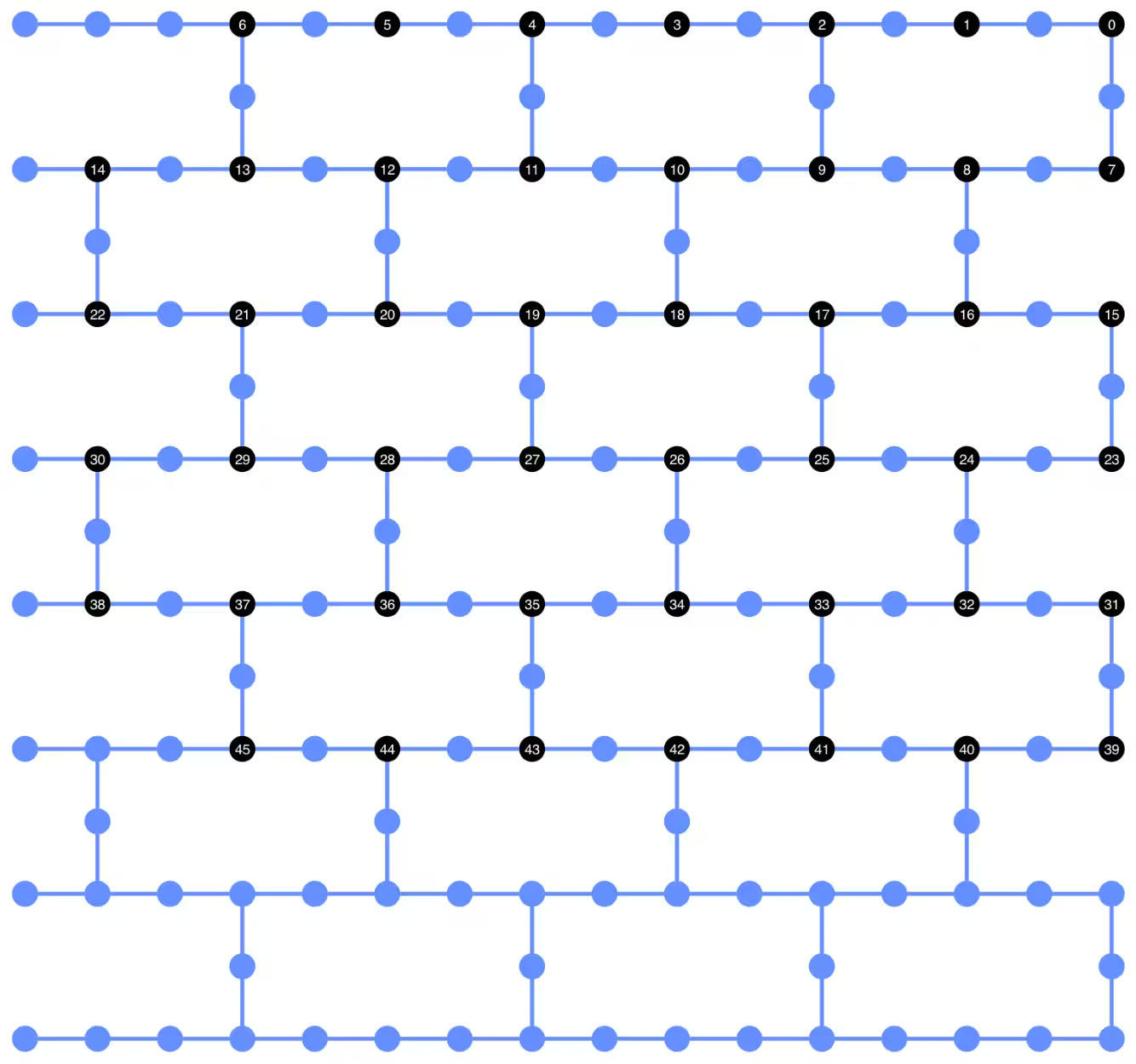
unitary_pubs = [(circ, params) for circ in unitary_isa_circuits]

We visualize the qubit layout of the transpiled unitary circuits. The black circles indicate the physical qubits used to transpile the unitary circuits and their indices correspond to the virtual qubit indices. By comparing this with the layout plotted for the dynamic circuits, we can confirm that the unitary circuits use the same set of physical qubits as the data qubits in the dynamic circuits.

plot_circuit_layout(
    unitary_isa_circuits[-1],
    backend,
    qubit_coordinates=_heron_coords_r2(),
    view="virtual",
)

Output:

We now add the DD sequence to the transpiled circuits and construct the corresponding PUBs for job submission.

pm_dd = PassManager(
    [
        ALAPScheduleAnalysis(target=backend.target),
        PadDynamicalDecoupling(
            dd_sequence=[
                XGate(),
                RZGate(np.pi),
                XGate(),
                RZGate(-np.pi),
            ],
            spacing=[1 / 4, 1 / 2, 0, 0, 1 / 4],
            target=backend.target,
        ),
    ]
)
 
unitary_isa_circuits_dd = pm_dd.run(unitary_isa_circuits)
unitary_pubs_dd = [(circ, params) for circ in unitary_isa_circuits_dd]

Compare two-qubit gate depth of unitary and dynamic circuits

# compare circuit depth of unitary and dynamic circuit implementations
unitary_depth = [
    unitary_isa_circuits[i].depth(lambda x: x.operation.num_qubits == 2)
    for i in range(len(unitary_isa_circuits))
]
 
dynamic_depth = [
    dynamic_isa_circuits[i].depth(lambda x: x.operation.num_qubits == 2)
    for i in range(len(dynamic_isa_circuits))
]
 
plt.plot(
    list(range(len(unitary_depth))),
    unitary_depth,
    label="unitary circuits",
    color="#be95ff",
)
plt.plot(
    list(range(len(dynamic_depth))),
    dynamic_depth,
    label="dynamic circuits",
    color="#ff7eb6",
)
plt.xlabel("Trotter steps")
plt.ylabel("Two-qubit depth")
plt.legend()

Output:

<matplotlib.legend.Legend at 0x374225760>

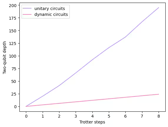
The main benefit of the measurement-based circuit is that, when implementing multiple ZZ interactions, the CX layers can be parallelized, and measurements can occur simultaneously. This is because all ZZ interactions commute, so the computation can be performed with measurement depth 1. After transpiling the circuits, we observe that the dynamic circuit approach yields a significantly shorter two-qubit depth than the standard unitary approach, with the caveat that the additional mid-circuit measurement and the classical feedforward themselves take time and introduce their own sources of errors.

Step 3: Execute using Qiskit primitives

Local testing mode

Before submitting the jobs to the hardware, we can run a small test simulation of the dynamic circuit using the local testing mode.

aer_sim = AerSimulator()
pm = generate_preset_pass_manager(backend=aer_sim, optimization_level=1)
circuit_dynamic_test.measure_all()
isa_qc = pm.run(circuit_dynamic_test)
with Batch(backend=aer_sim) as batch:
    sampler = Sampler(mode=batch)
    result = sampler.run([(isa_qc, params)]).result()
 
print(
    "Simulated average magnetization at trotter step = 1 at three theta values"
)
result[0].data["meas"].expectation_values(obs_dynamic_test[0])

Output:

Simulated average magnetization at trotter step = 1 at three theta values

array([ 0.16666667,  0.01855469, -0.13476562])

MPS simulation

For large circuits, we can use the matrix_product_state (MPS) simulator, which provides an approximate result to the expectation value according to the chosen bond dimension. We later use the MPS simulation results as the baseline to compare the results from the hardware.

# The MPS simulation below took approximately 7 minutes to run on a laptop with Apple M1 chip
 
mps_backend = AerSimulator(
    method="matrix_product_state",
    matrix_product_state_truncation_threshold=1e-5,
    matrix_product_state_max_bond_dimension=100,
)
mps_sampler = Aer_Sampler.from_backend(mps_backend)
 
shots = 4096
 
data_sim = []
for j in range(points):
    circ_list = [
        circ.assign_parameters([params[j]]) for circ in circuits_unitary
    ]
 
    mps_job = mps_sampler.run(circ_list, shots=shots)
    result = mps_job.result()
 
    point_data = [
        result[d].data["meas"].expectation_values(observables_unitary)
        for d in depths
    ]
 
    data_sim.append(point_data)  # data at one theta value
 
data_sim = np.array(data_sim)

With the circuits and observables prepared, we now execute them on hardware using the Sampler primitive.

Here we submit three jobs for unitary_pubs, dynamic_pubs, and dynamic_pubs_dd. Each is a list of parametrized circuits corresponding to nine different Trotter steps with three different $\theta$ parameters.

shots = 10000
 
with Batch(backend=backend) as batch:
    sampler = Sampler(mode=batch)
 
    sampler.options.experimental = {
        "execution": {
            "scheduler_timing": True
        },  # set to True to retrieve circuit timing info
    }
 
    job_unitary = sampler.run(unitary_pubs, shots=shots)
    print(f"unitary: {job_unitary.job_id()}")
 
    job_unitary_dd = sampler.run(unitary_pubs_dd, shots=shots)
    print(f"unitary_dd: {job_unitary_dd.job_id()}")
 
    job_dynamic = sampler.run(dynamic_pubs, shots=shots)
    print(f"dynamic: {job_dynamic.job_id()}")
 
    job_dynamic_dd = sampler.run(dynamic_pubs_dd, shots=shots)
    print(f"dynamic_dd: {job_dynamic_dd.job_id()}")
 
    job_dynamic_meas2 = sampler.run(dynamic_pubs_meas2, shots=shots)
    print(f"dynamic_meas2: {job_dynamic_meas2.job_id()}")
 
    job_dynamic_dd_meas2 = sampler.run(dynamic_pubs_dd_meas2, shots=shots)
    print(f"dynamic_dd_meas2: {job_dynamic_dd_meas2.job_id()}")

Output:

unitary: d5dtt0ldq8ts73fvbhj0
unitary: d5dtt11smlfc739onuag
dynamic: d5dtt1hsmlfc739onuc0
dynamic_dd: d5dtt25jngic73avdne0
dynamic_meas2: d5dtt2ldq8ts73fvbhm0
dynamic_dd_meas2: d5dtt2tjngic73avdnf0

Step 4: Post-process and return results in desired classical format

After the jobs have completed, we can retrieve the circuit duration from the job results metadata and visualize the circuit schedule information. To read more about visualizing a circuit's scheduling information, refer to this page.

# Circuit durations is reported in the unit of `dt` which can be retrieved from `Backend` object
unitary_durations = [
    job_unitary.result()[i].metadata["compilation"]["scheduler_timing"][
        "circuit_duration"
    ]
    for i in depths
]
 
dynamic_durations = [
    job_dynamic.result()[i].metadata["compilation"]["scheduler_timing"][
        "circuit_duration"
    ]
    for i in depths
]
 
dynamic_durations_meas2 = [
    job_dynamic_meas2.result()[i].metadata["compilation"]["scheduler_timing"][
        "circuit_duration"
    ]
    for i in depths
]
 
result_dd = job_dynamic_dd.result()[1]
circuit_schedule_dd = result_dd.metadata["compilation"]["scheduler_timing"][
    "timing"
]
 
# to visualize the circuit schedule, one can show the figure below
fig_dd = draw_circuit_schedule_timing(
    circuit_schedule=circuit_schedule_dd,
    included_channels=None,
    filter_readout_channels=False,
    filter_barriers=False,
    width=1000,
)
 
# Save to a file since the figure is large
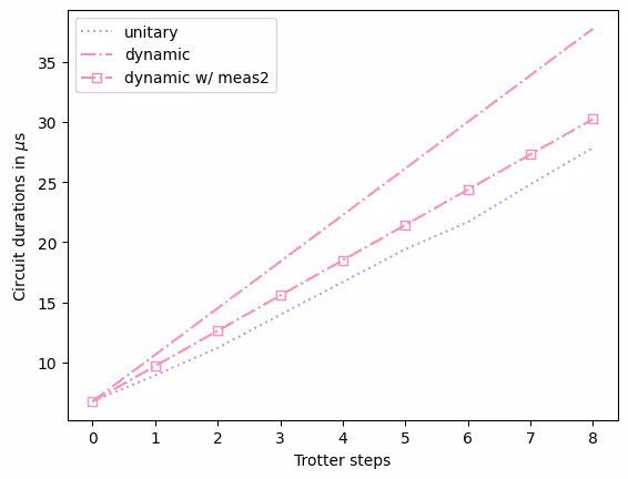
fig_dd.write_html("scheduler_timing_dd.html")

We plot the circuit durations for unitary circuits and the dynamic circuits. From the plot below, we can see that, despite the time needed for mid-circuit measurements and classical operations, dynamic circuit implementation with measure_2 results in comparable circuit durations as the unitary implementation.

# visualize circuit durations
 
 
def convert_dt_to_microseconds(circ_duration: List, backend_dt: float):
    dt = backend_dt * 1e6  # dt in microseconds
    return list(map(lambda x: x * dt, circ_duration))
 
 
dt = backend.target.dt
plt.plot(
    depths,
    convert_dt_to_microseconds(unitary_durations, dt),
    color="#be95ff",
    linestyle=":",
    label="unitary",
)
plt.plot(
    depths,
    convert_dt_to_microseconds(dynamic_durations, dt),
    color="#ff7eb6",
    linestyle="-.",
    label="dynamic",
)
plt.plot(
    depths,
    convert_dt_to_microseconds(dynamic_durations_meas2, dt),
    color="#ff7eb6",
    linestyle="-.",
    marker="s",
    mfc="none",
    label="dynamic w/ meas2",
)
 
plt.xlabel("Trotter steps")
plt.ylabel(r"Circuit durations in $\mu$s")
plt.legend()

Output:

<matplotlib.legend.Legend at 0x17f73c6e0>

After the jobs have completed, we retrieve the data below and compute the average magnetization estimated by the observables observables_unitary or observables_dynamic we constructed earlier.

runs = {
    "unitary": (
        job_unitary,
        [observables_unitary] * len(circuits_unitary),
    ),
    "unitary_dd": (
        job_unitary_dd,
        [observables_unitary] * len(circuits_unitary),
    ),
    # Omitting Dyn w/o DD and Dynamic w/ DD plots for better readability
    # "dynamic": (job_dynamic, observables_dynamic),
    # "dynamic_dd": (job_dynamic_dd, observables_dynamic),
    "dynamic_meas2": (job_dynamic_meas2, observables_dynamic),
    "dynamic_dd_meas2": (
        job_dynamic_dd_meas2,
        observables_dynamic,
    ),
}

data_dict = {}
for key, (job, obs) in runs.items():
    data = []
    for i in range(points):
        data.append(
            [
                job.result()[ind].data["meas"].expectation_values(obs[ind])[i]
                for ind in depths
            ]
        )
    data_dict[key] = data

Below we plot the spin magnetization as a function of the Trotter steps at different $\theta$ values, corresponding to different strengths of the local magnetic field. We plot both the pre-computed MPS simulation results for the unitary ideal circuits, together with the experimental results from the following:

running the unitary circuits with DD
running the dynamic circuits with DD and MidCircuitMeasure

plt.figure(figsize=(10, 6))
 
colors = ["#0f62fe", "#be95ff", "#ff7eb6"]
for i in range(points):
    plt.plot(
        depths,
        data_sim[i],
        color=colors[i],
        linestyle="solid",
        label=f"θ={pi_check(i*max_angle/(points-1))} (MPS)",
    )
    # plt.plot(
    #     depths,
    #     data_dict["unitary"][i],
    #     color=colors[i],
    #     linestyle=":",
    #     label=f"θ={pi_check(i*max_angle/(points-1))} (Unitary)",
    # )
 
    plt.plot(
        depths,
        data_dict["unitary_dd"][i],
        color=colors[i],
        marker="o",
        mfc="none",
        linestyle=":",
        label=f"θ={pi_check(i*max_angle/(points-1))} (Unitary w/DD)",
    )
 
    # Omitting Dyn w/o DD and Dynamic w/ DD plots for better readability
    # plt.plot(
    #     depths,
    #     data_dict["dynamic"][i],
    #     color=colors[i],
    #     linestyle="-.",
    #     label=f"θ={pi_check(i*max_angle/(points-1))} (Dyn w/o DD)",
    # )
    # plt.plot(
    #     depths,
    #     data_dict["dynamic_dd"][i],
    #     marker="D",
    #     mfc="none",
    #     color=colors[i],
    #     linestyle="-.",
    #     label=f"θ={pi_check(i*max_angle/(points-1))} (Dynamic w/ DD)",
    # )
 
    # plt.plot(
    #     depths,
    #     data_dict["dynamic_meas2"][i],
    #     color=colors[i],
    #     marker="s",
    #     mfc="none",
    #     linestyle=':',
    #     label=f"θ={pi_check(i*max_angle/(points-1))} (Dynamic w/ MidCircuitMeas)",
    # )
 
    plt.plot(
        depths,
        data_dict["dynamic_dd_meas2"][i],
        color=colors[i],
        marker="*",
        markersize=8,
        linestyle=":",
        label=f"θ={pi_check(i*max_angle/(points-1))} (Dynamic w/ DD & MidCircuitMeas)",
    )
 
 
plt.xlabel("Trotter steps", fontsize=16)
plt.ylabel("Average magnetization", fontsize=16)
plt.xticks(rotation=45)
handles, labels = plt.gca().get_legend_handles_labels()
plt.legend(
    handles,
    labels,
    loc="upper right",
    bbox_to_anchor=(1.46, 1.0),
    shadow=True,
    ncol=1,
)
plt.title(
    f"{hex_rows}x{hex_cols} hex ring, {num_qubits} data qubits, {len(ancilla)} ancilla qubits \n{backend.name}: Sampler"
)
plt.show()

Output:

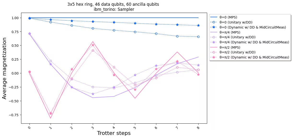
When we compare the experimental results with the simulation, we see that the dynamic circuit implementation (dotted line with stars) overall has better performance than the standard unitary implementation (dotted line with circles). In summary, we present dynamic circuits as a solution for simulating Ising spin models on a honeycomb lattice, a topology that is not native to the hardware. The dynamic circuit solution allows ZZ interactions between qubits that are not nearest neighbors, with a shorter two-qubit gate depth than using SWAP gates, at the cost of introducing extra ancilla qubits and classical feedforward operations.

References

[1] Quantum computing with Qiskit, by Javadi-Abhari, A., Treinish, M., Krsulich, K., Wood, C.J., Lishman, J., Gacon, J., Martiel, S., Nation, P.D., Bishop, L.S., Cross, A.W. and Johnson, B.R., 2024. arXiv preprint arXiv:2405.08810 (2024)

Simulation of kicked Ising Hamiltonian with dynamic circuits

Requirements

Set up

Step 1: Map classical inputs to a quantum circuit

Build unitary circuits

Build dynamic circuit implementation

Dynamical decoupling (DD) and support for stretch duration

Step 2: Optimize problem for hardware execution

Transpilation for dynamic circuits

Transpile using MidCircuitMeasure

Transpilation for unitary circuits

Compare two-qubit gate depth of unitary and dynamic circuits

Step 3: Execute using Qiskit primitives

Local testing mode

MPS simulation

Step 4: Post-process and return results in desired classical format

References

Dynamical decoupling (DD) and support for `stretch` duration

Transpile using `MidCircuitMeasure`