Quantum Phase Estimation with Q-CTRL's Qiskit Functions

Usage estimate: 40 seconds on a Heron r2 processor. (NOTE: This is an estimate only. Your runtime may vary.)

Background

Quantum Phase Estimation (QPE) is a foundational algorithm in quantum computing that forms the basis of many important applications such as Shor’s algorithm, quantum chemistry ground-state energy estimation, and eigenvalue problems. QPE estimates the phase $\varphi$ associated with an eigenstate of a unitary operator, encoded in the relation

$U \lvert \varphi \rangle = e^{2\pi i \varphi} \lvert \varphi \rangle,$

and determines it to a precision of $\epsilon = O(1/2^m)$ using $m$ counting qubits [1]. By preparing these qubits in superposition, applying controlled powers of $U$ , and then using the inverse Quantum Fourier Transform (QFT) to extract the phase into binary-encoded measurement outcomes, QPE produces a probability distribution peaked at bitstrings whose binary fractions approximate $\varphi$ . In the ideal case, the most likely measurement outcome directly corresponds to the binary expansion of the phase, while the probability of other outcomes decreases rapidly with the number of counting qubits. However, running deep QPE circuits on hardware presents challenges: the large number of qubits and entangling operations make the algorithm highly sensitive to decoherence and gate errors. This results in broadened and shifted distributions of bitstrings, masking the true eigenphase. As a consequence, the bitstring with the highest probability may no longer correspond to the correct binary expansion of $\varphi$ .

In this tutorial, we present an implementation of the QPE algorithm using Q-CTRL's Fire Opal error suppression and performance management tools, offered as a Qiskit Function (see the Fire Opal documentation). Fire Opal automatically applies advanced optimizations, including dynamical decoupling, qubit layout improvements, and error suppression techniques, resulting in higher-fidelity outcomes. These improvements bring hardware bitstring distributions closer to those obtained in noiseless simulations, so that you can reliably identify the correct eigenphase even under the effects of noise.

Requirements

Before starting this tutorial, be sure you have the following installed:

Qiskit SDK v1.4 or later, with visualization support ( pip install 'qiskit[visualization]' )
Qiskit Runtime v0.40 or later (pip install qiskit-ibm-runtime)
Qiskit Functions Catalog v0.9.0 (pip install qiskit-ibm-catalog)
Fire Opal SDK v9.0.2 or later (pip install fire-opal)
Q-CTRL Visualizer v8.0.2 or later (pip install qctrl-visualizer)

Setup

First, authenticate using your IBM Quantum API key. Then, select the Qiskit Function as follows. (This code assumes you've already saved your account to your local environment.)

from qiskit import QuantumCircuit
 
import numpy as np
import matplotlib.pyplot as plt
import qiskit
from qiskit import qasm2
from qiskit_aer import AerSimulator
from qiskit_ibm_runtime import QiskitRuntimeService
from qiskit_ibm_runtime import SamplerV2 as Sampler
from qiskit.transpiler.preset_passmanagers import generate_preset_pass_manager
import qctrlvisualizer as qv
from qiskit_ibm_catalog import QiskitFunctionsCatalog
 
plt.style.use(qv.get_qctrl_style())

catalog = QiskitFunctionsCatalog(channel="ibm_quantum_platform")
 
# Access Function
perf_mgmt = catalog.load("q-ctrl/performance-management")

Step 1: Map classical inputs to a quantum problem

In this tutorial, we illustrate QPE to recover the eigenphase of a known single-qubit unitary. The unitary whose phase we want to estimate is the single-qubit phase gate applied to the target qubit:

U(\theta)= \begin{pmatrix} 1 & 0\\[2pt] 0 & e^{i\theta} \end{pmatrix} = e^{i\theta\,|1\rangle\!\langle 1|}.

We prepare its eigenstate $|\psi\rangle=|1\rangle$ . Because $|1\rangle$ is an eigenvector of $U(\theta)$ with eigenvalue $e^{i\theta}$ , the eigenphase to be estimated is:

\varphi = \frac{\theta}{2\pi} \pmod{1}

We set $\theta=\tfrac{1}{6}\cdot 2\pi$ , so the ground-truth phase is $\varphi=1/6$ . The QPE circuit implements the controlled powers $U^{2^k}$ by applying controlled phase rotations with angles $\theta\cdot2^k$ , then applies the inverse QFT to the counting register and measures it. The resulting bitstrings concentrate around the binary representation of $1/6$ .

The circuit uses $m$ counting qubits (to set the estimation precision) plus one target qubit. We begin by defining the building blocks needed to implement QPE: the Quantum Fourier Transform (QFT) and its inverse, utility functions to map between decimal and binary fractions of the eigenphase, and helpers to normalize raw counts into probabilities for comparing simulation and hardware results.

def inverse_quantum_fourier_transform(quantum_circuit, number_of_qubits):
    """
    Apply an inverse Quantum Fourier Transform the first `number_of_qubits` qubits in the
    `quantum_circuit`.
    """
    for qubit in range(number_of_qubits // 2):
        quantum_circuit.swap(qubit, number_of_qubits - qubit - 1)
    for j in range(number_of_qubits):
        for m in range(j):
            quantum_circuit.cp(-np.pi / float(2 ** (j - m)), m, j)
        quantum_circuit.h(j)
    return quantum_circuit

def bitstring_count_to_probabilities(data, shot_count):
    """
    This function turns an unsorted dictionary of bitstring counts into a sorted dictionary
    of probabilities.
    """
    # Turn the bitstring counts into probabilities.
    probabilities = {
        bitstring: bitstring_count / shot_count
        for bitstring, bitstring_count in data.items()
    }
 
    sorted_probabilities = dict(
        sorted(probabilities.items(), key=lambda x: x[1], reverse=True)
    )
 
    return sorted_probabilities

Step 2: Optimize problem for quantum hardware execution

We build the QPE circuit by preparing the counting qubits in superposition, applying controlled phase rotations to encode the target eigenphase, and finishing with an inverse QFT before measurement.

def quantum_phase_estimation_benchmark_circuit(
    number_of_counting_qubits, phase
):
    """
    Create the circuit for quantum phase estimation.
 
    Parameters
    ----------
    number_of_counting_qubits : The number of qubits in the circuit.
    phase : The desired phase.
 
    Returns
    -------
    QuantumCircuit
        The quantum phase estimation circuit for `number_of_counting_qubits` qubits.
    """
    qc = QuantumCircuit(
        number_of_counting_qubits + 1, number_of_counting_qubits
    )
    target = number_of_counting_qubits
 
    # |1> eigenstate for the single-qubit phase gate
    qc.x(target)
 
    # Hadamards on counting register
    for q in range(number_of_counting_qubits):
        qc.h(q)
 
    # ONE controlled phase per counting qubit: cp(phase * 2**k)
    for k in range(number_of_counting_qubits):
        qc.cp(phase * (1 << k), k, target)
 
    qc.barrier()
 
    # Inverse QFT on counting register
    inverse_quantum_fourier_transform(qc, number_of_counting_qubits)
 
    qc.barrier()
    for q in range(number_of_counting_qubits):
        qc.measure(q, q)
    return qc

Step 3: Execute using Qiskit primitives

We set the number of shots and qubits for the experiment, and encode the target phase $\varphi = 1/6$ using $m$ binary digits. With these parameters, we build the QPE circuit that will be executed on simulation, default hardware, and Fire Opal–enhanced backends.

shot_count = 10000
num_qubits = 35
phase = (1 / 6) * 2 * np.pi
circuits_quantum_phase_estimation = (
    quantum_phase_estimation_benchmark_circuit(
        number_of_counting_qubits=num_qubits, phase=phase
    )
)

Run MPS simulation

First, we generate a reference distribution using the matrix_product_state simulator and convert the counts into normalized probabilities for later comparison with hardware results.

# Run the algorithm on the IBM Aer simulator.
aer_simulator = AerSimulator(method="matrix_product_state")
 
# Transpile the circuits for the simulator.
transpiled_circuits = qiskit.transpile(
    circuits_quantum_phase_estimation, aer_simulator
)

simulated_result = (
    aer_simulator.run(transpiled_circuits, shots=shot_count)
    .result()
    .get_counts()
)

simulated_result_probabilities = []
 
simulated_result_probabilities.append(
    bitstring_count_to_probabilities(
        simulated_result,
        shot_count=shot_count,
    )
)

Run on hardware

service = QiskitRuntimeService()
backend = service.least_busy(operational=True, simulator=False)
 
pm = generate_preset_pass_manager(backend=backend, optimization_level=3)
isa_circuits = pm.run(circuits_quantum_phase_estimation)

# Run the algorithm with IBM default.
sampler = Sampler(backend)
 
# Run all circuits using Qiskit Runtime.
ibm_default_job = sampler.run([isa_circuits], shots=shot_count)

Run on hardware with Fire Opal

# Run the circuit using the sampler
fire_opal_job = perf_mgmt.run(
    primitive="sampler",
    pubs=[qasm2.dumps(circuits_quantum_phase_estimation)],
    backend_name=backend.name,
    options={"default_shots": shot_count},
)

Step 4: Post-process and return result in desired classical format

# Retrieve results.
ibm_default_result = ibm_default_job.result()
ibm_default_probabilities = []
 
for idx, pub_result in enumerate(ibm_default_result):
    ibm_default_probabilities.append(
        bitstring_count_to_probabilities(
            pub_result.data.c0.get_counts(),
            shot_count=shot_count,
        )
    )

fire_opal_result = fire_opal_job.result()
 
fire_opal_probabilities = []
for idx, pub_result in enumerate(fire_opal_result):
    fire_opal_probabilities.append(
        bitstring_count_to_probabilities(
            pub_result.data.c0.get_counts(),
            shot_count=shot_count,
        )
    )

data = {
    "simulation": simulated_result_probabilities,
    "default": ibm_default_probabilities,
    "fire_opal": fire_opal_probabilities,
}

def plot_distributions(
    data,
    number_of_counting_qubits,
    top_k=None,
    by="prob",
    shot_count=None,
):
    def nrm(d):
        s = sum(d.values())
        return {k: (v / s if s else 0.0) for k, v in d.items()}
 
    def as_float(d):
        return {k: float(v) for k, v in d.items()}
 
    def to_space(d):
        if by == "prob":
            return nrm(as_float(d))
        else:
            if shot_count and 0.99 <= sum(d.values()) <= 1.01:
                return {
                    k: v * float(shot_count) for k, v in as_float(d).items()
                }
            else:
                return as_float(d)
 
    def topk(d, k):
        items = sorted(d.items(), key=lambda kv: kv[1], reverse=True)
        return items[: (k or len(d))]
 
    phase = "1/6"
 
    sim = to_space(data["simulation"])
    dft = to_space(data["default"])
    qct = to_space(data["fire_opal"])
 
    correct = max(sim, key=sim.get) if sim else None
    print("Correct result:", correct)
 
    sim_items = topk(sim, top_k)
    dft_items = topk(dft, top_k)
    qct_items = topk(qct, top_k)
 
    sim_keys, y_sim = zip(*sim_items) if sim_items else ([], [])
    dft_keys, y_dft = zip(*dft_items) if dft_items else ([], [])
    qct_keys, y_qct = zip(*qct_items) if qct_items else ([], [])
 
    fig, axes = plt.subplots(3, 1, layout="constrained")
    ylab = "Probabilities"
 
    def panel(ax, keys, ys, title, color):
        x = np.arange(len(keys))
        bars = ax.bar(x, ys, color=color)
        ax.set_title(title)
        ax.set_ylabel(ylab)
        ax.set_xticks(x)
        ax.set_xticklabels(keys, rotation=90)
        ax.set_xlabel("Bitstrings")
        if correct in keys:
            i = keys.index(correct)
            bars[i].set_edgecolor("black")
            bars[i].set_linewidth(2)
        return max(ys, default=0.0)
 
    c_sim, c_dft, c_qct = (
        qv.QCTRL_STYLE_COLORS[5],
        qv.QCTRL_STYLE_COLORS[1],
        qv.QCTRL_STYLE_COLORS[0],
    )
    m1 = panel(axes[0], list(sim_keys), list(y_sim), "Simulation", c_sim)
    m2 = panel(axes[1], list(dft_keys), list(y_dft), "Default", c_dft)
    m3 = panel(axes[2], list(qct_keys), list(y_qct), "Q-CTRL", c_qct)
 
    for ax, m in zip(axes, (m1, m2, m3)):
        ax.set_ylim(0, 1.05 * (m or 1.0))
 
    for ax in axes:
        ax.label_outer()
    fig.suptitle(
        rf"{number_of_counting_qubits} counting qubits, $2\pi\varphi$={phase}"
    )
    fig.set_size_inches(20, 10)
    plt.show()

experiment_index = 0
phase_index = 0
 
distributions = {
    "simulation": data["simulation"][phase_index],
    "default": data["default"][phase_index],
    "fire_opal": data["fire_opal"][phase_index],
}
 
plot_distributions(
    distributions, num_qubits, top_k=100, by="prob", shot_count=shot_count
)

Output:

Correct result: 00101010101010101010101010101010101

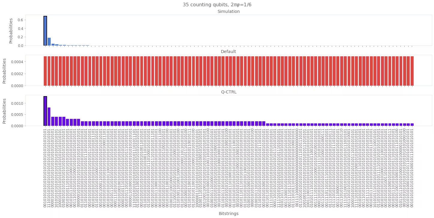
The simulation sets the baseline for the correct eigenphase. Default hardware runs show noise that obscures this result, as noise spreads probability across many incorrect bitstrings. With Q-CTRL Performance Management the distribution becomes sharper and the correct outcome is recovered, enabling reliable QPE at this scale.

References

[1] Lecture 7: Phase Estimation and Factoring. IBM Quantum Learning - Fundamentals of quantum algorithms. Retrieved October 3, 2025.

Tutorial survey

Please take a minute to provide feedback on this tutorial. Your insights will help us improve our content offerings and user experience.

Link to survey