Improving energy estimation of a fermionic lattice model with SQD
Usage estimate: 9 seconds on IBM Aachen (NOTE: This is an estimate only. Your runtime may vary.)
Background
In this tutorial, we show how to use sample-based quantum diagonalization (SQD) to estimate the ground state energy of a fermionic lattice model. Specifically, we study the one-dimensional single-impurity Anderson model (SIAM), which is used to describe magnetic impurities embedded in metals.
This tutorial follows a similar workflow to the related tutorial Sample-based quantum diagonalization of a chemistry Hamiltonian. However, a key difference lies in how the quantum circuits are built. The other tutorial uses a heuristic variational ansatz, which is appealing for chemistry Hamiltonians with potentially millions of interaction terms. On the other hand, this tutorial uses circuits that approximate time evolution by the Hamiltonian. Such circuits can be deep, which makes this approach better for applications to lattice models. The state vectors prepared by these circuits form the basis for a Krylov subspace, and as a result, the algorithm provably and efficiently converges to the ground state, under suitable assumptions.
The approach used in this tutorial can be viewed as a combination of the techniques used in SQD and Krylov quantum diagonalization (KQD). The combined approach is sometimes referred to as sample-based Krylov quantum diagonalization (SQKD). See Krylov quantum diagonalization of lattice Hamiltonians for a tutorial on the KQD method.
This tutorial is based on the work "Quantum-Centric Algorithm for Sample-Based Krylov Diagonalization", which can be referred to for more details.
Single-impurity Anderson model (SIAM)
The one-dimensional SIAM Hamiltonian is a sum of three terms:
where
Here, are the fermionic creation/annihilation operators for the bath site with spin , are creation/annihilation operators for the impurity mode, and . , , and are real numbers describing the hopping, on-site, hybridization interactions, and is a real number specifying the chemical potential.
Note that the Hamiltonian is a specific instance of the generic interaction-electron Hamiltonian,
where consists of one-body terms, which are quadratic in the fermionic creation and annihilation operators, and consists of two-body terms, which are quartic. For the SIAM,
and contains the rest of the terms in the Hamiltonian. In order to represent the Hamiltonian programmatically, we store the matrix and the tensor .
Position and momentum bases
Due to the approximate translational symmetry in , we don't expect the ground state to be sparse in the position basis (the orbital basis in which the Hamiltonian is specified above). The performance of SQD is guaranteed only if the ground state is sparse, that is, it has significant weight on only a small number of computational basis states. To improve the sparsity of the ground state, we perform the simulation in the orbital basis in which is diagonal. We call this basis the momentum basis. Because is a quadratic fermionic Hamiltonian, it can be efficiently diagonalized by an orbital rotation.
Approximate time evolution by the Hamiltonian
To approximate time evolution by the Hamiltonian, we use a second order Trotter-Suzuki decomposition,
Under the Jordan-Wigner transformation, time evolution by amounts to a single CPhase gate between the spin-up and spin-down orbitals at the impurity site. Because is a quadratic fermionic Hamiltonian, time evolution by amounts to an orbital rotation.
The Krylov basis states , where is the dimension of the Krylov subspace, are formed by repeated application of a single Trotter step, so
In the following SQD-based workflow, we will sample from this set of circuits and postprocess the combined set of bitstrings with SQD. This approach contrasts with the one used in the related tutorial Sample-based quantum diagonalization of a chemistry Hamiltonian, where samples were drawn from a single heuristic variational circuit.
Requirements
Before starting this tutorial, ensure that you have the following installed:
- Qiskit SDK 1.0 or later with visualization support (
pip install 'qiskit[visualization]') - Qiskit Runtime 0.22 or later (
pip install qiskit-ibm-runtime) - SQD Qiskit addon 0.11 or later (
pip install qiskit-addon-sqd) - ffsim (
pip install ffsim)
Step 1: Map problem to a quantum circuit
First, we generate the SIAM Hamiltonian in the position basis. The Hamiltonian is represented by the matrix and the tensor . Then, we rotate it to the momentum basis. In the position basis, we place the impurity at the first site. However, when we rotate to the momentum basis, we move the impurity to a central site to facilitate interactions with other orbitals.
import numpy as np
def siam_hamiltonian(
norb: int,
hopping: float,
onsite: float,
hybridization: float,
chemical_potential: float,
) -> tuple[np.ndarray, np.ndarray]:
"""Hamiltonian for the single-impurity Anderson model."""
# Place the impurity on the first site
impurity_orb = 0
# One body matrix elements in the "position" basis
h1e = np.zeros((norb, norb))
np.fill_diagonal(h1e[:, 1:], -hopping)
np.fill_diagonal(h1e[1:, :], -hopping)
h1e[impurity_orb, impurity_orb + 1] = -hybridization
h1e[impurity_orb + 1, impurity_orb] = -hybridization
h1e[impurity_orb, impurity_orb] = chemical_potential
# Two body matrix elements in the "position" basis
h2e = np.zeros((norb, norb, norb, norb))
h2e[impurity_orb, impurity_orb, impurity_orb, impurity_orb] = onsite
return h1e, h2e
def momentum_basis(norb: int) -> np.ndarray:
"""Get the orbital rotation to change from the position to the momentum basis."""
n_bath = norb - 1
# Orbital rotation that diagonalizes the bath (non-interacting system)
hopping_matrix = np.zeros((n_bath, n_bath))
np.fill_diagonal(hopping_matrix[:, 1:], -1)
np.fill_diagonal(hopping_matrix[1:, :], -1)
_, vecs = np.linalg.eigh(hopping_matrix)
# Expand to include impurity
orbital_rotation = np.zeros((norb, norb))
# Impurity is on the first site
orbital_rotation[0, 0] = 1
orbital_rotation[1:, 1:] = vecs
# Move the impurity to the center
new_index = n_bath // 2
perm = np.r_[1 : (new_index + 1), 0, (new_index + 1) : norb]
orbital_rotation = orbital_rotation[:, perm]
return orbital_rotation
def rotated(
h1e: np.ndarray, h2e: np.ndarray, orbital_rotation: np.ndarray
) -> tuple[np.ndarray, np.ndarray]:
"""Rotate the orbital basis of a Hamiltonian."""
h1e_rotated = np.einsum(
"ab,Aa,Bb->AB",
h1e,
orbital_rotation,
orbital_rotation.conj(),
optimize="greedy",
)
h2e_rotated = np.einsum(
"abcd,Aa,Bb,Cc,Dd->ABCD",
h2e,
orbital_rotation,
orbital_rotation.conj(),
orbital_rotation,
orbital_rotation.conj(),
optimize="greedy",
)
return h1e_rotated, h2e_rotated
# Total number of spatial orbitals, including the bath sites and the impurity
# This should be an even number
norb = 20
# System is half-filled
nelec = (norb // 2, norb // 2)
# One orbital is the impurity, the rest are bath sites
n_bath = norb - 1
# Hamiltonian parameters
hybridization = 1.0
hopping = 1.0
onsite = 10.0
chemical_potential = -0.5 * onsite
# Generate Hamiltonian in position basis
h1e, h2e = siam_hamiltonian(
norb=norb,
hopping=hopping,
onsite=onsite,
hybridization=hybridization,
chemical_potential=chemical_potential,
)
# Rotate to momentum basis
orbital_rotation = momentum_basis(norb)
h1e_momentum, h2e_momentum = rotated(h1e, h2e, orbital_rotation.T.conj())
# In the momentum basis, the impurity is placed in the center
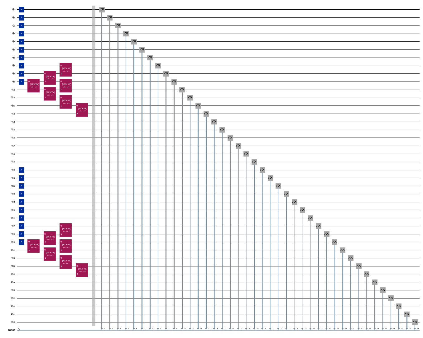
impurity_index = n_bath // 2Next, we generate the circuits to produce the Krylov basis states. For each spin species, the initial state is given by the superposition of all possible excitations of the three electrons closest to the Fermi level into the 4 closest empty modes starting from the state , and realized by the application of seven XXPlusYYGates. The time-evolved states are produced by successive applications of a second-order Trotter step.
For a more detailed description of this model and how the circuits are designed, refer to "Quantum-Centric Algorithm for Sample-Based Krylov Diagonalization".
from typing import Sequence

import ffsim
import scipy
from qiskit import QuantumCircuit, QuantumRegister
from qiskit.circuit import CircuitInstruction, Qubit
from qiskit.circuit.library import CPhaseGate, XGate, XXPlusYYGate


def prepare_initial_state(qubits: Sequence[Qubit], norb: int, nocc: int):
    """Prepare initial state."""
    x_gate = XGate()
    rot = XXPlusYYGate(0.5 * np.pi, -0.5 * np.pi)
    for i in range(nocc):
        yield CircuitInstruction(x_gate, [qubits[i]])
        yield CircuitInstruction(x_gate, [qubits[norb + i]])
    for i in range(3):
        for j in range(nocc - i - 1, nocc + i, 2):
            yield CircuitInstruction(rot, [qubits[j], qubits[j + 1]])
            yield CircuitInstruction(
                rot, [qubits[norb + j], qubits[norb + j + 1]]
            )
    yield CircuitInstruction(rot, [qubits[j + 1], qubits[j + 2]])
    yield CircuitInstruction(
        rot, [qubits[norb + j + 1], qubits[norb + j + 2]]
    )


def trotter_step(
    qubits: Sequence[Qubit],
    time_step: float,
    one_body_evolution: np.ndarray,
    h2e: np.ndarray,
    impurity_index: int,
    norb: int,
):
    """A Trotter step."""
    # Assume the two-body interaction is just the on-site interaction of the impurity
    onsite = h2e[
        impurity_index, impurity_index, impurity_index, impurity_index
    ]
    # Two-body evolution for half the time
    yield CircuitInstruction(
        CPhaseGate(-0.5 * time_step * onsite),
        [qubits[impurity_index], qubits[norb + impurity_index]],
    )
    # One-body evolution for the full time
    yield CircuitInstruction(
        ffsim.qiskit.OrbitalRotationJW(norb, one_body_evolution), qubits
    )
    # Two-body evolution for half the time
    yield CircuitInstruction(
        CPhaseGate(-0.5 * time_step * onsite),
        [qubits[impurity_index], qubits[norb + impurity_index]],
    )


# Time step
time_step = 0.2
# Number of Krylov basis states
krylov_dim = 8

# Initialize circuit
qubits = QuantumRegister(2 * norb, name="q")
circuit = QuantumCircuit(qubits)

# Generate initial state
for instruction in prepare_initial_state(qubits, norb=norb, nocc=norb // 2):
    circuit.append(instruction)
circuit.measure_all()

# Create list of circuits, starting with the initial state circuit
circuits = [circuit.copy()]

# Add time evolution circuits to the list
one_body_evolution = scipy.linalg.expm(-1j * time_step * h1e_momentum)
for i in range(krylov_dim - 1):
    # Remove measurements
    circuit.remove_final_measurements()
    # Append another Trotter step
    for instruction in trotter_step(
        qubits,
        time_step,
        one_body_evolution,
        h2e_momentum,
        impurity_index,
        norb,
    ):
        circuit.append(instruction)
    # Measure qubits
    circuit.measure_all()
    # Add a copy of the circuit to the list
circuits.append(circuit.copy())circuits[0].draw("mpl", scale=0.4, fold=-1)Output:
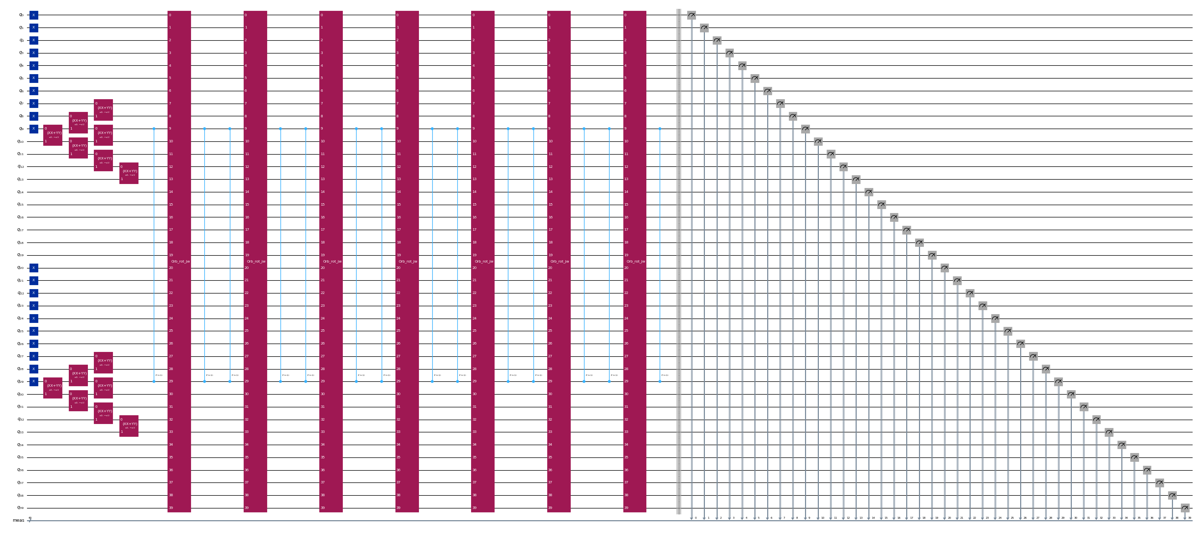
circuits[-1].draw("mpl", scale=0.4, fold=-1)Output:
Step 2: Optimize problem for quantum execution
Now that we have created the circuits, we can optimize them for a target hardware. We pick the least busy QPU with at least 127 qubits. Check out the Qiskit IBM Runtime docs for more information.
from qiskit_ibm_runtime import QiskitRuntimeService

service = QiskitRuntimeService()
backend = service.least_busy(
    operational=True, simulator=False, min_num_qubits=127
)
print(f"Using backend {backend.name}")
Output:
Using backend ibm_fez
Now, we use Qiskit to transpile the circuits to the target backend.
from qiskit.transpiler import generate_preset_pass_manager

pass_manager = generate_preset_pass_manager(
    optimization_level=3, backend=backend
)
isa_circuits = pass_manager.run(circuits)
Step 3: Execute by using Qiskit primitives
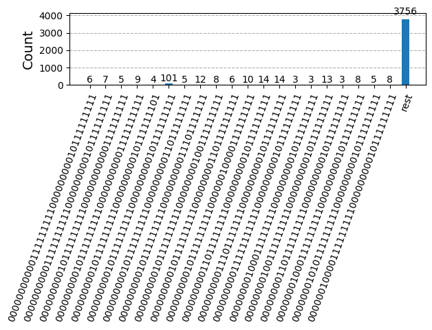
After optimizing the circuits for hardware execution, we are ready to run them on the target hardware and collect samples for ground state energy estimation. After using the Sampler primitive to sample bitstrings from each circuit, we combine all of the results into a single counts dictionary and plot the top 20 most commonly sampled bitstrings.
from qiskit.visualization import plot_histogram
from qiskit_ibm_runtime import SamplerV2 as Sampler

# Sample from the circuits
sampler = Sampler(backend)
job = sampler.run(isa_circuits, shots=500)
from qiskit.primitives import BitArray
# Combine the counts from the individual Trotter circuits
bit_array = BitArray.concatenate_shots(
[result.data.meas for result in job.result()]
)
plot_histogram(bit_array.get_counts(), number_to_keep=20)Output:
Step 4: Post-process and return result to desired classical format
Now, we run the SQD algorithm using the diagonalize_fermionic_hamiltonian function. See the API documentation for explanations of the arguments to this function.
from qiskit_addon_sqd.fermion import (
    SCIResult,
    diagonalize_fermionic_hamiltonian,
)

# List to capture intermediate results
result_history = []


def callback(results: list[SCIResult]):
    result_history.append(results)
    iteration = len(result_history)
    print(f"Iteration {iteration}")
    for i, result in enumerate(results):
        print(f"\tSubsample {i}")
        print(f"\t\tEnergy: {result.energy}")
        print(
            f"\t\tSubspace dimension: {np.prod(result.sci_state.amplitudes.shape)}"
        )


rng = np.random.default_rng(24)
result = diagonalize_fermionic_hamiltonian(
    h1e_momentum,
    h2e_momentum,
    bit_array,
    samples_per_batch=100,
    norb=norb,
    nelec=nelec,
    num_batches=3,
    max_iterations=5,
    symmetrize_spin=True,
    callback=callback,
    seed=rng,
)
Output:
Iteration 1
	Subsample 0
		Energy: -28.61321893815165
		Subspace dimension: 10609
	Subsample 1
		Energy: -28.628985564542244
		Subspace dimension: 13924
	Subsample 2
		Energy: -28.620151775558114
		Subspace dimension: 10404
Iteration 2
	Subsample 0
		Energy: -28.656893066053115
		Subspace dimension: 34225
	Subsample 1
		Energy: -28.65277622004119
		Subspace dimension: 38416
	Subsample 2
		Energy: -28.670856034959165
		Subspace dimension: 39601
Iteration 3
	Subsample 0
		Energy: -28.684787675404362
		Subspace dimension: 42436
	Subsample 1
		Energy: -28.676984757118426
		Subspace dimension: 50176
	Subsample 2
		Energy: -28.671581704249885
		Subspace dimension: 40804
Iteration 4
	Subsample 0
		Energy: -28.6859683054753
		Subspace dimension: 47961
	Subsample 1
		Energy: -28.69418206537316
		Subspace dimension: 51529
	Subsample 2
		Energy: -28.686083516445752
		Subspace dimension: 51529
Iteration 5
	Subsample 0
		Energy: -28.694665630711178
		Subspace dimension: 50625
	Subsample 1
		Energy: -28.69505984237118
		Subspace dimension: 47524
	Subsample 2
		Energy: -28.6942873883992
		Subspace dimension: 48841
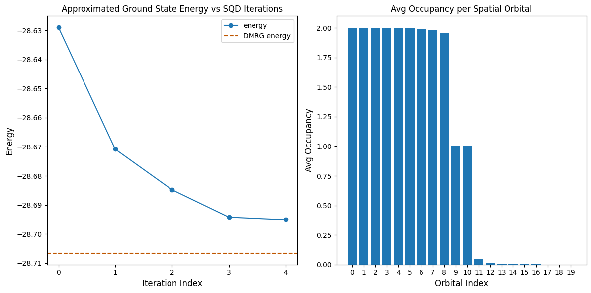
The following code cell plots the results. The first plot shows the computed energy as a function of the number of configuration recovery iterations, and the second plot shows the average occupancy of each spatial orbital after the final iteration. For the reference energy, we use the results of a DMRG calculation that was performed separately.
import matplotlib.pyplot as plt

dmrg_energy = -28.70659686

min_es = [
    min(result, key=lambda res: res.energy).energy
    for result in result_history
]
min_id, min_e = min(enumerate(min_es), key=lambda x: x[1])

# Data for energies plot
x1 = range(len(result_history))

# Data for avg spatial orbital occupancy
y2 = np.sum(result.orbital_occupancies, axis=0)
x2 = range(len(y2))

fig, axs = plt.subplots(1, 2, figsize=(12, 6))

# Plot energies
axs[0].plot(x1, min_es, label="energy", marker="o")
axs[0].set_xticks(x1)
axs[0].set_xticklabels(x1)
axs[0].axhline(
    y=dmrg_energy, color="#BF5700", linestyle="--", label="DMRG energy"
)
axs[0].set_title("Approximated Ground State Energy vs SQD Iterations")
axs[0].set_xlabel("Iteration Index", fontdict={"fontsize": 12})
axs[0].set_ylabel("Energy", fontdict={"fontsize": 12})
axs[0].legend()

# Plot orbital occupancy
axs[1].bar(x2, y2, width=0.8)
axs[1].set_xticks(x2)
axs[1].set_xticklabels(x2)
axs[1].set_title("Avg Occupancy per Spatial Orbital")
axs[1].set_xlabel("Orbital Index", fontdict={"fontsize": 12})
axs[1].set_ylabel("Avg Occupancy", fontdict={"fontsize": 12})

print(f"Reference (DMRG) energy: {dmrg_energy:.5f}")
print(f"SQD energy: {min_e:.5f}")
print(f"Absolute error: {abs(min_e - dmrg_energy):.5f}")
plt.tight_layout()
plt.show()
Output:
Reference (DMRG) energy: -28.70660
SQD energy: -28.69506
Absolute error: 0.01154
Verifying the energy
The energy returned by SQD is guaranteed to be an upper bound to the true ground state energy. The value of the energy can be verified because SQD also returns the coefficients of the state vector approximating the ground state. You can compute the energy from the state vector using its 1- and 2-particle reduced density matrices, as demonstrated in the following code cell.
rdm1 = result.sci_state.rdm(rank=1, spin_summed=True)
rdm2 = result.sci_state.rdm(rank=2, spin_summed=True)

energy = np.sum(h1e_momentum * rdm1) + 0.5 * np.sum(h2e_momentum * rdm2)

print(f"Recomputed energy: {energy:.5f}")
Output:
Recomputed energy: -28.69506