Variational quantum eigensolver
Usage estimate: 73 minutes on IBM Kyiv (NOTE: This is an estimate only. Your runtime may vary.)
Background
Variational quantum algorithms are promising candidate hybrid-algorithms for observing quantum computation utility on noisy near-term devices. Variational algorithms are characterized by the use of a classical optimization algorithm to iteratively update a parameterized trial solution, or "ansatz". Chief among these methods is the Variational Quantum Eigensolver (VQE) that aims to solve for the ground state of a given Hamiltonian represented as a linear combination of Pauli terms, with an ansatz circuit where the number of parameters to optimize over is polynomial in the number of qubits. Given that the size of the full solution vector is exponential in the number of qubits, successful minimization using VQE requires, in general, additional problem-specific information to define the structure of the ansatz circuit.
Executing a VQE algorithm requires the following components:
- Hamiltonian and ansatz (problem specification)
- Qiskit Runtime estimator
- Classical optimizer
Although the Hamiltonian and ansatz require domain-specific knowledge to construct, these details are immaterial to the Runtime, and we can execute a wide class of VQE problems in the same manner.
Requirements
Before starting this tutorial, ensure that you have the following installed:
- Qiskit SDK 1.0 or later, with visualization support (
pip install 'qiskit[visualization]') - Qiskit Runtime 0.22 or later(
pip install qiskit-ibm-runtime)
Setup
import matplotlib.pyplot as plt
import numpy as np
from scipy.optimize import minimize

from qiskit.circuit.library import efficient_su2
from qiskit.quantum_info import SparsePauliOp
from qiskit.transpiler.preset_passmanagers import generate_preset_pass_manager

from qiskit_ibm_runtime import QiskitRuntimeService, Session
from qiskit_ibm_runtime import EstimatorV2 as Estimator
Step 1: Map classical inputs to a quantum problem
Although the problem instance in question for the VQE algorithm can come from a variety of domains, the form for execution through Qiskit Runtime is the same. Qiskit provides a convenience class for expressing Hamiltonians in Pauli form, and a collection of widely used ansatz circuits in the qiskit.circuit.library.
This example Hamiltonian is derived from a quantum chemistry problem.
# To run on hardware, select the backend with the fewest number of jobs in the queue
service = QiskitRuntimeService()
backend = service.least_busy(
    operational=True, simulator=False, min_num_qubits=127
)
hamiltonian = SparsePauliOp.from_list(
[("YZ", 0.3980), ("ZI", -0.3980), ("ZZ", -0.0113), ("XX", 0.1810)]
)Our choice of ansatz is the efficient_su2 that, by default, linearly entangles qubits, making it ideal for quantum hardware with limited connectivity.
ansatz = efficient_su2(hamiltonian.num_qubits)
ansatz.decompose().draw("mpl", style="iqp")
Output:
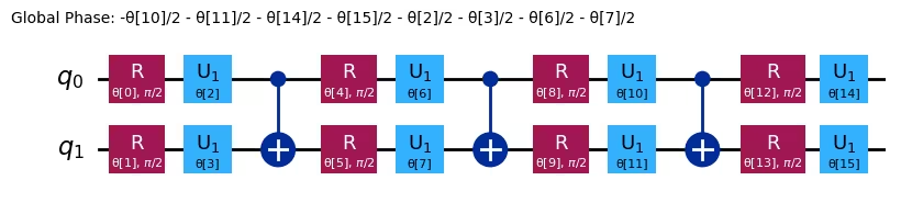
From the previous figure we see that our ansatz circuit is defined by a vector of parameters, , with the total number given by:
num_params = ansatz.num_parameters
num_params
Output:
16
Step 2: Optimize problem for quantum hardware execution
To reduce the total job execution time, Qiskit primitives only accept circuits (ansatz) and observables (Hamiltonian) that conform to the instructions and connectivity supported by the target QPU (referred to as instruction set architecture (ISA) circuits and observables).
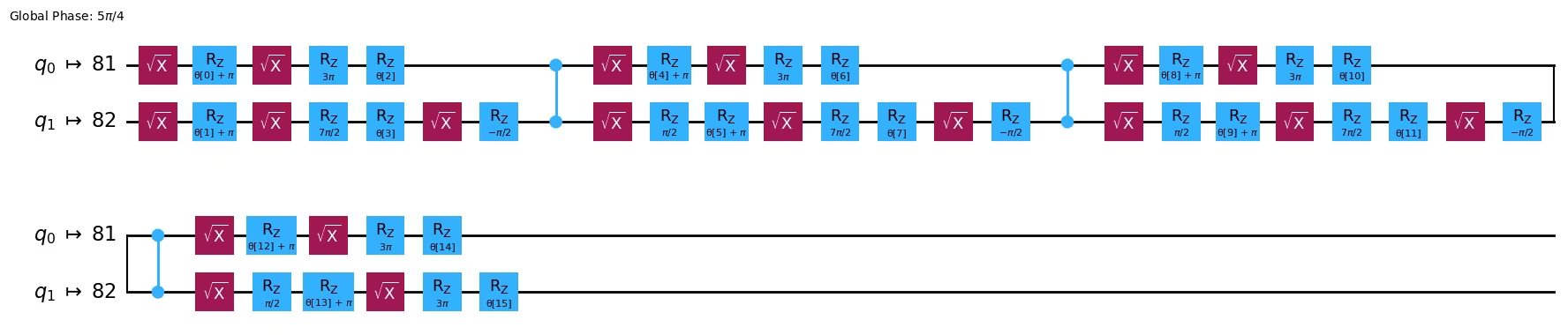
ISA circuit
Schedule a series of qiskit.transpiler passes to optimize the circuit for a selected backend and make it compatible with the backend's ISA. This can be easily done with a preset pass manager from qiskit.transpiler and its optimization_level parameter.
The lowest optimization level does the minimum needed to get the circuit running on the device; it maps the circuit qubits to the device qubits and adds swap gates to allow all two-qubit operations. The highest optimization level is much smarter and uses lots of tricks to reduce the overall gate count. Since multi-qubit gates have high error rates and qubits decohere over time, the shorter circuits should give better results.
target = backend.target
pm = generate_preset_pass_manager(target=target, optimization_level=3)

ansatz_isa = pm.run(ansatz)ansatz_isa.draw(output="mpl", idle_wires=False, style="iqp")Output:
ISA observable
Transform the Hamiltonian to make it backend-compatible before running jobs with Runtime Estimator V2. Perform the transformation by using the apply_layout method of SparsePauliOp object.
hamiltonian_isa = hamiltonian.apply_layout(layout=ansatz_isa.layout)Step 3: Execute using Qiskit primitives
Like many classical optimization problems, the solution to a VQE problem can be formulated as minimization of a scalar cost function. By definition, VQE looks to find the ground state solution to a Hamiltonian by optimizing the ansatz circuit parameters to minimize the expectation value (energy) of the Hamiltonian. With the Qiskit Runtime Estimator directly taking a Hamiltonian and parameterized ansatz, and returning the necessary energy, the cost function for a VQE instance is quite simple.
Note that the run() method of Qiskit Runtime EstimatorV2 takes an iterable of primitive unified blocs (PUBs). Each PUB is an iterable in the format (circuit, observables, parameter_values: Optional, precision: Optional).
def cost_func(params, ansatz, hamiltonian, estimator):
    """Return estimate of energy from estimator

    Parameters:
        params (ndarray): Array of ansatz parameters
        ansatz (QuantumCircuit): Parameterized ansatz circuit
        hamiltonian (SparsePauliOp): Operator representation of Hamiltonian
        estimator (EstimatorV2): Estimator primitive instance
        cost_history_dict: Dictionary for storing intermediate results

    Returns:
        float: Energy estimate
    """
    pub = (ansatz, [hamiltonian], [params])
    result = estimator.run(pubs=[pub]).result()
    energy = result[0].data.evs[0]

    cost_history_dict["iters"] += 1
    cost_history_dict["prev_vector"] = params
    cost_history_dict["cost_history"].append(energy)
    print(
        f"Iters. done: {cost_history_dict['iters']} [Current cost: {energy}]"
    )

    return energy
Note that, in addition to the array of optimization parameters that must be the first argument, we use additional arguments to pass the terms needed in the cost function. We also access a global variable called cost_history_dict within this function. This dictionary stores the current vector at each iteration, for example in case you need to restart the routine due to failure, and also returns the current iteration number and average time per iteration.
cost_history_dict = {
    "prev_vector": None,
    "iters": 0,
    "cost_history": [],
}
We can now use a classical optimizer of our choice to minimize the cost function. Here, we use the COBYLA routine from SciPy through the minimize function. Note that when running on real quantum hardware, the choice of optimizer is important, as not all optimizers handle noisy cost function landscapes equally well.
To begin the routine, specify a random initial set of parameters:
x0 = 2 * np.pi * np.random.random(num_params)x0Output:
array([2.51632747, 0.41779892, 5.85800259, 4.83749838, 3.20828874,
       5.23058321, 0.23909191, 5.93347588, 0.98307886, 5.8564212 ,
       3.41519817, 2.07444879, 0.7790487 , 0.72421971, 1.09848722,
       3.31663941])
Because we are sending a large number of jobs that we would like to execute iteratively, we use a Session to execute all the generated circuits in one block. Here args is the standard SciPy way to supply the additional parameters needed by the cost function.
with Session(backend=backend) as session:
    estimator = Estimator(mode=session)
    estimator.options.default_shots = 10000

    res = minimize(
        cost_func,
        x0,
        args=(ansatz_isa, hamiltonian_isa, estimator),
        method="cobyla",
    )
Output:
Iters. done: 1 [Current cost: -0.41297466987766457]
Iters. done: 2 [Current cost: -0.4074417945791059]
Iters. done: 3 [Current cost: -0.3547606824167446]
Iters. done: 4 [Current cost: -0.28168907720107683]
Iters. done: 5 [Current cost: -0.4578159863650208]
Iters. done: 6 [Current cost: -0.3086594190935841]
Iters. done: 7 [Current cost: -0.15483382641187454]
Iters. done: 8 [Current cost: -0.5349854031388536]
Iters. done: 9 [Current cost: -0.3895567829431972]
Iters. done: 10 [Current cost: -0.4820250378135054]
Iters. done: 11 [Current cost: -0.18395917730188865]
Iters. done: 12 [Current cost: -0.5311791591751455]
Iters. done: 13 [Current cost: -0.49602925858832053]
Iters. done: 14 [Current cost: -0.3482916173440449]
Iters. done: 15 [Current cost: -0.5668230348151325]
Iters. done: 16 [Current cost: -0.521882967057639]
Iters. done: 17 [Current cost: -0.26976382760304113]
Iters. done: 18 [Current cost: -0.051127606468041646]
Iters. done: 19 [Current cost: -0.5213490424900524]
Iters. done: 20 [Current cost: -0.5519837695254404]
Iters. done: 21 [Current cost: -0.5729754281424254]
Iters. done: 22 [Current cost: -0.5369152381529558]
Iters. done: 23 [Current cost: -0.54862310847568]
Iters. done: 24 [Current cost: -0.5843821664926876]
Iters. done: 25 [Current cost: -0.58018047409157]
Iters. done: 26 [Current cost: -0.5153040139793709]
Iters. done: 27 [Current cost: -0.5950601168931274]
Iters. done: 28 [Current cost: -0.5919884877771185]
Iters. done: 29 [Current cost: -0.6295788565552562]
Iters. done: 30 [Current cost: -0.5909207781822071]
Iters. done: 31 [Current cost: -0.6029330648206948]
Iters. done: 32 [Current cost: -0.5731453720567535]
Iters. done: 33 [Current cost: -0.6017005875653386]
Iters. done: 34 [Current cost: -0.6061613567553928]
Iters. done: 35 [Current cost: -0.5527009036762591]
Iters. done: 36 [Current cost: -0.6174016810951264]
Iters. done: 37 [Current cost: -0.5331013786620393]
Iters. done: 38 [Current cost: -0.6174716771227629]
Iters. done: 39 [Current cost: -0.5256692009209388]
Iters. done: 40 [Current cost: -0.5936376314600634]
Iters. done: 41 [Current cost: -0.6174496293908639]
Iters. done: 42 [Current cost: -0.6415583284028612]
Iters. done: 43 [Current cost: -0.6568655223778936]
Iters. done: 44 [Current cost: -0.6252111792327242]
Iters. done: 45 [Current cost: -0.6588010261150293]
Iters. done: 46 [Current cost: -0.6031535817582718]
Iters. done: 47 [Current cost: -0.6448573357168782]
Iters. done: 48 [Current cost: -0.6314357577602281]
Iters. done: 49 [Current cost: -0.6310360137350473]
Iters. done: 50 [Current cost: -0.6311716934542182]
Iters. done: 51 [Current cost: -0.6195122556941205]
Iters. done: 52 [Current cost: -0.6052709851652176]
Iters. done: 53 [Current cost: -0.6353235502797585]
Iters. done: 54 [Current cost: -0.6172917549286481]
Iters. done: 55 [Current cost: -0.6157291352122161]
Iters. done: 56 [Current cost: -0.6250258800660834]
Iters. done: 57 [Current cost: -0.6238737928804968]
Iters. done: 58 [Current cost: -0.6331336376123765]
Iters. done: 59 [Current cost: -0.6174795053010914]
Iters. done: 60 [Current cost: -0.6286114171740883]
Iters. done: 61 [Current cost: -0.6289541704111539]
Iters. done: 62 [Current cost: -0.6214988287789815]
Iters. done: 63 [Current cost: -0.6349088785327752]
Iters. done: 64 [Current cost: -0.6434368257074341]
Iters. done: 65 [Current cost: -0.6435758714276368]
Iters. done: 66 [Current cost: -0.6392426194852974]
Iters. done: 67 [Current cost: -0.6395388664428873]
Iters. done: 68 [Current cost: -0.6288383465181286]
Iters. done: 69 [Current cost: -0.6396744408945687]
Iters. done: 70 [Current cost: -0.6313800275882947]
Iters. done: 71 [Current cost: -0.6253344175379661]
Iters. done: 72 [Current cost: -0.6157835899181318]
Iters. done: 73 [Current cost: -0.6335140148162095]
Iters. done: 74 [Current cost: -0.6314904503216308]
Iters. done: 75 [Current cost: -0.6400032416620431]
Iters. done: 76 [Current cost: -0.6467193690082172]
Iters. done: 77 [Current cost: -0.6274062557744253]
Iters. done: 78 [Current cost: -0.6382220718392321]
Iters. done: 79 [Current cost: -0.6353720791573834]
Iters. done: 80 [Current cost: -0.6559597232796966]
Iters. done: 81 [Current cost: -0.6483482402979868]
Iters. done: 82 [Current cost: -0.6362917844251428]
Iters. done: 83 [Current cost: -0.638689906716738]
Iters. done: 84 [Current cost: -0.6398683206762882]
Iters. done: 85 [Current cost: -0.6411425890703265]
Iters. done: 86 [Current cost: -0.6420124690404581]
Iters. done: 87 [Current cost: -0.6361424203927645]
Iters. done: 88 [Current cost: -0.6304230811374153]
Iters. done: 89 [Current cost: -0.6460686380415002]
Iters. done: 90 [Current cost: -0.6393627867774831]
Iters. done: 91 [Current cost: -0.6353801863066766]
Iters. done: 92 [Current cost: -0.6370827028067767]
Iters. done: 93 [Current cost: -0.6367252584729324]
Iters. done: 94 [Current cost: -0.6369091807759274]
Iters. done: 95 [Current cost: -0.6358923615709814]
Iters. done: 96 [Current cost: -0.6374055046408706]
Iters. done: 97 [Current cost: -0.6449879432951772]
Iters. done: 98 [Current cost: -0.646341931913156]
Iters. done: 99 [Current cost: -0.6329474251488447]
Iters. done: 100 [Current cost: -0.640483532296447]
Iters. done: 101 [Current cost: -0.6387821271169515]
Iters. done: 102 [Current cost: -0.6444401199777418]
Iters. done: 103 [Current cost: -0.624905121027599]
Iters. done: 104 [Current cost: -0.6254651227936383]
Iters. done: 105 [Current cost: -0.6350106349636292]
Iters. done: 106 [Current cost: -0.6452221411408458]
Iters. done: 107 [Current cost: -0.6510959797011343]
Iters. done: 108 [Current cost: -0.6335108244050601]
Iters. done: 109 [Current cost: -0.6463731459675923]
Iters. done: 110 [Current cost: -0.6453116341043271]
Iters. done: 111 [Current cost: -0.6500434300085539]
Iters. done: 112 [Current cost: -0.6498155030176934]
Iters. done: 113 [Current cost: -0.6165876514864352]
Iters. done: 114 [Current cost: -0.6379032301303812]
Iters. done: 115 [Current cost: -0.6238652143915986]
Iters. done: 116 [Current cost: -0.6303015369454892]
Iters. done: 117 [Current cost: -0.6387276591694434]
Iters. done: 118 [Current cost: -0.6216154977895596]
Iters. done: 119 [Current cost: -0.6254429094384901]
Iters. done: 120 [Current cost: -0.6244723070534346]
Iters. done: 121 [Current cost: -0.6331274845209857]
Iters. done: 122 [Current cost: -0.6320092007865726]
Iters. done: 123 [Current cost: -0.6280195555442015]
Iters. done: 124 [Current cost: -0.633118817842713]
Iters. done: 125 [Current cost: -0.6545316861761059]
Iters. done: 126 [Current cost: -0.6109521608105805]
Iters. done: 127 [Current cost: -0.6413687240373942]
Iters. done: 128 [Current cost: -0.6329171488537345]
Iters. done: 129 [Current cost: -0.6508873536148351]
Iters. done: 130 [Current cost: -0.6343396180590694]
Iters. done: 131 [Current cost: -0.6453833725535618]
Iters. done: 132 [Current cost: -0.6142726913357903]
Iters. done: 133 [Current cost: -0.6209357951339112]
Iters. done: 134 [Current cost: -0.6316232515088392]
Iters. done: 135 [Current cost: -0.6534320416334607]
Iters. done: 136 [Current cost: -0.6403781274445913]
Iters. done: 137 [Current cost: -0.6472281981296323]
Iters. done: 138 [Current cost: -0.6560563807840072]
Iters. done: 139 [Current cost: -0.6381191598219642]
Iters. done: 140 [Current cost: -0.635047673191689]
Iters. done: 141 [Current cost: -0.6346354679202391]
Iters. done: 142 [Current cost: -0.6426649674647372]
Iters. done: 143 [Current cost: -0.643370774702743]
Iters. done: 144 [Current cost: -0.6429365799217991]
Iters. done: 145 [Current cost: -0.641164172799006]
Iters. done: 146 [Current cost: -0.634701203143904]
At the terminus of this routine we have a result in the standard SciPy OptimizeResult format. From this we see that it took nfev number of cost function evaluations to obtain the solution vector of parameter angles (x) that, when plugged into the ansatz circuit, yield the approximate ground state solution we were looking for.
resOutput:
 message: Optimization terminated successfully.
 success: True
  status: 1
     fun: -0.634701203143904
       x: [ 2.581e+00  4.153e-01 ...  1.070e+00  3.123e+00]
    nfev: 146
   maxcv: 0.0
Step 4: Post-process and return result in desired classical format
If the procedure terminates correctly, then the prev_vector and iters values in our cost_history_dict dictionary should be equal to the solution vector and total number of function evaluations, respectively. This is easy to verify:
all(cost_history_dict["prev_vector"] == res.x)Output:
True
cost_history_dict["iters"] == res.nfevOutput:
False
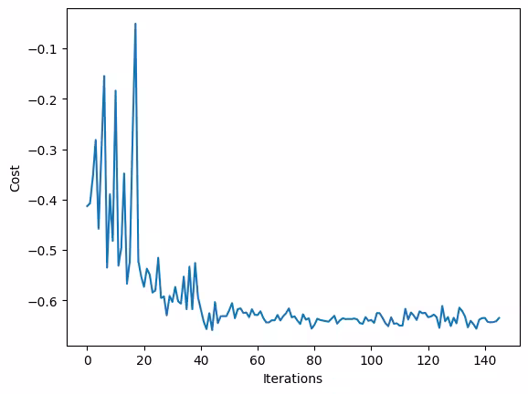
We can also now view the progress toward convergence as monitored by the cost history at each iteration:
fig, ax = plt.subplots()
ax.plot(range(cost_history_dict["iters"]), cost_history_dict["cost_history"])
ax.set_xlabel("Iterations")
ax.set_ylabel("Cost")
plt.draw()
Output:
Tutorial survey
Please take one minute to provide feedback on this tutorial. Your insights will help us improve our content offerings and user experience.
© IBM Corp., 2024, 2025