Sample-based quantum diagonalization of a chemistry Hamiltonian

Usage estimate: under 1 minute on ibm_kingston (NOTE: This is an estimate only. Your runtime may vary.)

Background

In this tutorial, we show how to post-process noisy quantum samples to find an approximation to the ground state of the nitrogen molecule $\text{N}_2$ at equilibrium bond length, using the sample-based quantum diagonalization (SQD) algorithm, for samples taken from a 36-qubit quantum circuit (32 system qubits + 4 ancilla qubits). A Qiskit-based implementation is available in the SQD Qiskit addons, more details can be found in the corresponding docs with a simple example to get started. SQD is a technique for finding eigenvalues and eigenvectors of quantum operators, such as a quantum system Hamiltonian, using quantum and distributed classical computing together. Classical distributed computing is used to process samples obtained from a quantum processor, and to project and diagonalize a target Hamiltonian in a subspace spanned by them. This allows SQD to be robust to samples corrupted by quantum noise and deal with large Hamiltonians, such as chemistry Hamiltonians with millions of interaction terms, beyond the reach of any exact diagonalization methods. An SQD-based workflow has the following steps:

1. Choose a circuit ansatz and apply it on a quantum computer to a reference state (in this case, the Hartree-Fock state).
2. Sample bitstrings from the resulting quantum state.
3. Run the self-consistent configuration recovery procedure on the bitstrings to obtain the approximation to the ground state.

SQD is known to work well when the target eigenstate is sparse: the wave function is supported in a set of basis states $\mathcal{S} = \{|x\rangle \}$ whose size does not increase exponentially with the size of the problem.

Quantum chemistry

The properties of molecules are largely determined by the structure of the electrons within them. As fermionic particles, electrons can be described using a mathematical formalism called second quantization. The idea is that there are a number of orbitals, each of which can be either empty or occupied by a fermion. A system of $N$ orbitals is described by a set of fermionic annihilation operators $\{\hat{a}_p\}_{p=1}^N$ that satisfy the fermionic anticommutation relations,

The adjoint $\hat{a}_p^\dagger$ is called a creation operator.

So far, our exposition has not accounted for spin, which is a fundamental property of fermions. When accounting for spin, the orbitals come in pairs called spatial orbitals. Each spatial orbital is composed of two spin orbitals, one that is labeled "spin-$\alpha$" and one that is labeled "spin-$\beta$". We then write $\hat{a}_{p\sigma}$ for the annihilation operator associated with the spin-orbital with spin $\sigma$ ($\sigma \in \{\alpha, \beta\}$) in spatial orbital $p$. If we take $N$ to be the number of spatial orbitals, then there are a total of $2N$ spin-orbitals. The Hilbert space of this system is spanned by $2^{2N}$ orthonormal basis vectors labeled with two-part bitstrings $\lvert z \rangle = \lvert z_\beta z_\alpha \rangle = \lvert z_{\beta, N} \cdots z_{\beta, 1} z_{\alpha, N} \cdots z_{\alpha, 1} \rangle$.

The Hamiltonian of a molecular system can be written as

where the $h_{pr}$ and $h_{prqs}$ are complex numbers called molecular integrals that can be calculated from the specification of the molecule using a computer program. In this tutorial, we compute the integrals using the PySCF software package.

For details about how the molecular Hamiltonian is derived, consult a textbook on quantum chemistry (for example, Modern Quantum Chemistry by Szabo and Ostlund). For a high-level explanation of how quantum chemistry problems are mapped onto quantum computers, check out the lecture Mapping Problems to Qubits from Qiskit Global Summer School 2024.

Local unitary cluster Jastrow (LUCJ) ansatz

SQD requires a quantum circuit ansatz to draw samples from. In this tutorial, we'll use the local unitary cluster Jastrow (LUCJ) ansatz due to its combination of physical motivation and hardware-friendliness.

The LUCJ ansatz is a specialized form of the general unitary cluster Jastrow (UCJ) ansatz, which has the form

where $\lvert \Phi_0 \rangle$ is a reference state, often taken to be the Hartree-Fock state, and the $\hat{K}_\mu$ and $\hat{J}_\mu$ have the form

where we have defined the number operator

The operator $e^{\hat{K}_\mu}$ is an orbital rotation, which can be implemented using known algorithms in linear depth and using linear connectivity. Implementing the $e^{i \mathcal{J}_k}$ term of the UCJ ansatz requires either all-to-all connectivity or the use of a fermionic swap network, making it challenging for noisy pre-fault-tolerant quantum processors that have limited connectivity. The idea of the local UCJ ansatz is to impose sparsity constraints on the $\mathbf{J}^{\alpha\alpha}$ and $\mathbf{J}^{\alpha\beta}$ matrices which allow them to be implemented in constant depth on qubit topologies with limited connectivity. The constraints are specified by a list of indices indicating which matrix entries in the upper triangle are allowed to be nonzero (since the matrices are symmetric, only the upper triangle needs to be specified). These indices can be interpreted as pairs of orbitals that are allowed to interact.

As an example, consider a square lattice qubit topology. We can place the $\alpha$ and $\beta$ orbitals in parallel lines on the lattice, with connections between these lines forming "rungs" of a ladder shape, like this:

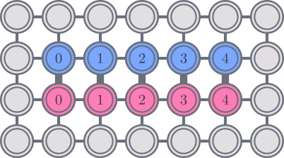
With this setup, orbitals with the same spin are connected with a line topology, while orbitals with different spins are connected when they share the same spatial orbital. This yields the following index constraints on the $\mathbf{J}$ matrices:

In other words, if the $\mathbf{J}$ matrices are nonzero only at the specified indices in the upper triangle, then the $e^{i \mathcal{J}_k}$ term can be implemented on a square topology without using any swap gates, in constant depth. Of course, imposing such constraints on the ansatz makes it less expressive, so more ansatz repetitions may be required.

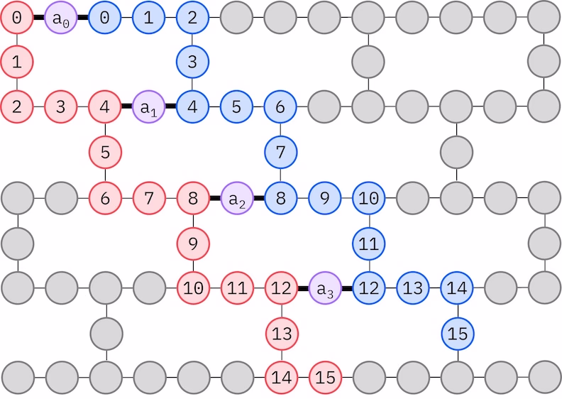
The IBM hardware has a heavy-hex lattice qubit topology, in which case we can adopt a "zig-zag" pattern, depicted below. In this pattern, orbitals with the same spin are mapped to qubits with a line topology (red and blue circles), and a connection between orbitals of different spin is present at every 4th spatial orbital, with the connection being facilitated by an ancilla qubit (purple circles). In this case, the index constraints are

Self-consistent configuration recovery

The self-consistent configuration recovery procedure is designed to extract as much signal as possible from noisy quantum samples. Because the molecular Hamiltonian conserves particle number and spin Z, it makes sense to choose a circuit ansatz that also conserves these symmetries. When applied to the Hartree-Fock state, the resulting state has a fixed particle number and spin Z in the noiseless setting. Therefore, the spin-$\alpha$ and spin-$\beta$ halves of any bitstring sampled from this state should have the same Hamming weight as in the Hartree-Fock state. Due to the presence of noise in current quantum processors, some measured bitstrings will violate this property. A simple form of postselection would discard these bitstrings, but this is wasteful because those bitstrings might still contain some signal. The self-consistent recovery procedure attempts to recover some of that signal in post-processing. The procedure is iterative and requires as input an estimate of the average occupancies of each orbital in the ground state, which is first computed from the raw samples. The procedure is run in a loop, and each iteration has the following steps:

1. For each bitstring that violates the specified symmetries, flip its bits with a probabilistic procedure designed to bring the bitstring closer to the current estimate of the average orbital occupancies, to obtain a new bitstring.
2. Collect all of the old and new bitstrings that satisfy the symmetries, and subsample subsets of a fixed size, chosen in advance.
3. For each subset of bitstrings, project the Hamiltonian into the subspace spanned by the corresponding basis vectors (see the previous section for a description of these basis vectors), and compute a ground state estimate of the projected Hamiltonian on a classical computer.
4. Update the estimate of the average orbital occupancies with the ground state estimate with the lowest energy.

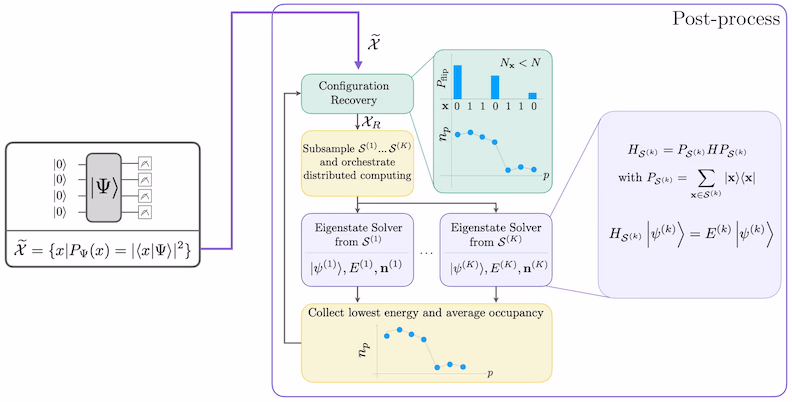
SQD workflow diagram

The SQD workflow is depicted in the following diagram:

Requirements

Before starting this tutorial, ensure that you have the following installed:

• Qiskit SDK 1.0 or later with visualization support (pip install 'qiskit[visualization]')
• Qiskit Runtime 0.22 or later (pip install qiskit-ibm-runtime)
• SQD Qiskit addon 0.11 or later (pip install qiskit-addon-sqd)
• ffsim (pip install ffsim)

Setup

import pyscf
import pyscf.cc
import pyscf.mcscf
import ffsim
import numpy as np
import matplotlib.pyplot as plt
 
from qiskit import QuantumCircuit, QuantumRegister
from qiskit.transpiler.preset_passmanagers import generate_preset_pass_manager
 
from qiskit_ibm_runtime import QiskitRuntimeService
from qiskit_ibm_runtime import SamplerV2 as Sampler

Step 1: Map classical inputs to a quantum problem

In this tutorial, we will find an approximation to the ground state of the molecule at equilibrium in the 6-31G basis set. First, we specify the molecule and its properties.

# Specify molecule properties
open_shell = False
spin_sq = 0
 
# Build N2 molecule
mol = pyscf.gto.Mole()
mol.build(
    atom=[["N", (0, 0, 0)], ["N", (1.0, 0, 0)]],
    basis="6-31g",
    symmetry="Dooh",
)
 
# Define active space
n_frozen = 2
active_space = range(n_frozen, mol.nao_nr())
 
# Get molecular integrals
scf = pyscf.scf.RHF(mol).run()
num_orbitals = len(active_space)
n_electrons = int(sum(scf.mo_occ[active_space]))
num_elec_a = (n_electrons + mol.spin) // 2
num_elec_b = (n_electrons - mol.spin) // 2
cas = pyscf.mcscf.CASCI(scf, num_orbitals, (num_elec_a, num_elec_b))
mo = cas.sort_mo(active_space, base=0)
hcore, nuclear_repulsion_energy = cas.get_h1cas(mo)
eri = pyscf.ao2mo.restore(1, cas.get_h2cas(mo), num_orbitals)
 
# Compute exact energy
exact_energy = cas.run().e_tot

Output:

converged SCF energy = -108.835236570775
CASCI E = -109.046671778080  E(CI) = -32.8155692383188  S^2 = 0.0000000

Before constructing the LUCJ ansatz circuit, we first perform a CCSD calculation in the following code cell. The $t_1$ and $t_2$ amplitudes from this calculation will be used to initialize the parameters of the ansatz.

# Get CCSD t2 amplitudes for initializing the ansatz
ccsd = pyscf.cc.CCSD(
    scf, frozen=[i for i in range(mol.nao_nr()) if i not in active_space]
).run()
t1 = ccsd.t1
t2 = ccsd.t2

Output:

E(CCSD) = -109.0398256929734  E_corr = -0.2045891221988307

Now, we use ffsim to create the ansatz circuit. Since our molecule has a closed-shell Hartree-Fock state, we use the spin-balanced variant of the UCJ ansatz, UCJOpSpinBalanced. We pass interaction pairs appropriate for a heavy-hex lattice qubit topology (see the background section on the LUCJ ansatz).

n_reps = 1
alpha_alpha_indices = [(p, p + 1) for p in range(num_orbitals - 1)]
alpha_beta_indices = [(p, p) for p in range(0, num_orbitals, 4)]
 
ucj_op = ffsim.UCJOpSpinBalanced.from_t_amplitudes(
    t2=t2,
    t1=t1,
    n_reps=n_reps,
    interaction_pairs=(alpha_alpha_indices, alpha_beta_indices),
)
 
nelec = (num_elec_a, num_elec_b)
 
# create an empty quantum circuit
qubits = QuantumRegister(2 * num_orbitals, name="q")
circuit = QuantumCircuit(qubits)
 
# prepare Hartree-Fock state as the reference state and append it to the quantum circuit
circuit.append(ffsim.qiskit.PrepareHartreeFockJW(num_orbitals, nelec), qubits)
 
# apply the UCJ operator to the reference state
circuit.append(ffsim.qiskit.UCJOpSpinBalancedJW(ucj_op), qubits)
circuit.measure_all()

Step 2: Optimize problem for quantum hardware execution

Next, we optimize the circuit for a target hardware.

service = QiskitRuntimeService()
backend = service.least_busy(
    operational=True, simulator=False, min_num_qubits=127
)

We recommend the following steps to optimize the ansatz and make it hardware-compatible.

• Select physical qubits (initial_layout) from the target hardware that adheres to the zig-zag pattern described above. Laying out qubits in this pattern leads to an efficient hardware-compatible circuit with less gates.
• Generate a staged pass manager using the generate_preset_pass_manager function from qiskit with your choice of backend and initial_layout.
• Set the pre_init stage of your staged pass manager to ffsim.qiskit.PRE_INIT. ffsim.qiskit.PRE_INIT includes qiskit transpiler passes that decompose gates into orbital rotations and then merges the orbital rotations, resulting in fewer gates in the final circuit.
• Run the pass manager on your circuit.

spin_a_layout = [
    0,
    14,
    18,
    19,
    20,
    33,
    39,
    40,
    41,
    53,
    60,
    61,
    62,
    72,
    81,
    82,
]
spin_b_layout = [2, 3, 4, 15, 22, 23, 24, 34, 43, 44, 45, 54, 64, 65, 66, 73]
initial_layout = spin_a_layout + spin_b_layout
 
pass_manager = generate_preset_pass_manager(
    optimization_level=3, backend=backend, initial_layout=initial_layout
)
 
# without PRE_INIT passes
isa_circuit = pass_manager.run(circuit)
print(f"Gate counts (w/o pre-init passes): {isa_circuit.count_ops()}")
 
# with PRE_INIT passes
# We will use the circuit generated by this pass manager for hardware execution
pass_manager.pre_init = ffsim.qiskit.PRE_INIT
isa_circuit = pass_manager.run(circuit)
print(f"Gate counts (w/ pre-init passes): {isa_circuit.count_ops()}")

Output:

Gate counts (w/o pre-init passes): OrderedDict({'sx': 5780, 'rz': 3536, 'cz': 2600, 'x': 288, 'measure': 32, 'barrier': 1})
Gate counts (w/ pre-init passes): OrderedDict({'sx': 4225, 'rz': 2274, 'cz': 1832, 'x': 145, 'measure': 32, 'barrier': 1})

Step 3: Execute using Qiskit primitives

After optimizing the circuit for hardware execution, we are ready to run it on the target hardware and collect samples for ground state energy estimation. As we only have one circuit, we will use Qiskit Runtime's Job execution mode and execute our circuit.

sampler = Sampler(mode=backend)
job = sampler.run([isa_circuit], shots=100_000)

primitive_result = job.result()
pub_result = primitive_result[0]

Step 4: Post-process and return result in desired classical format

Now, we estimate the ground state energy of the Hamiltonian using the diagonalize_fermionic_hamiltonian function. This function performs the self-consistent configuration recovery procedure to iteratively refine the noisy quantum samples to improve the energy estimate. We pass a callback function so that we can save the intermediate results for later analysis. See the API documentation for explanations of the arguments to diagonalize_fermionic_hamiltonian.

from functools import partial
 
from qiskit_addon_sqd.fermion import (
    SCIResult,
    diagonalize_fermionic_hamiltonian,
    solve_sci_batch,
)
 
# SQD options
energy_tol = 1e-3
occupancies_tol = 1e-3
max_iterations = 5
 
# Eigenstate solver options
num_batches = 3
samples_per_batch = 300
symmetrize_spin = True
carryover_threshold = 1e-4
max_cycle = 200
 
# Pass options to the built-in eigensolver. If you just want to use the defaults,
# you can omit this step, in which case you would not specify the sci_solver argument
# in the call to diagonalize_fermionic_hamiltonian below.
sci_solver = partial(solve_sci_batch, spin_sq=0.0, max_cycle=max_cycle)
 
# List to capture intermediate results
result_history = []
 
 
def callback(results: list[SCIResult]):
    result_history.append(results)
    iteration = len(result_history)
    print(f"Iteration {iteration}")
    for i, result in enumerate(results):
        print(f"\tSubsample {i}")
        print(f"\t\tEnergy: {result.energy + nuclear_repulsion_energy}")
        print(
            f"\t\tSubspace dimension: {np.prod(result.sci_state.amplitudes.shape)}"
        )
 
 
result = diagonalize_fermionic_hamiltonian(
    hcore,
    eri,
    pub_result.data.meas,
    samples_per_batch=samples_per_batch,
    norb=num_orbitals,
    nelec=nelec,
    num_batches=num_batches,
    energy_tol=energy_tol,
    occupancies_tol=occupancies_tol,
    max_iterations=max_iterations,
    sci_solver=sci_solver,
    symmetrize_spin=symmetrize_spin,
    carryover_threshold=carryover_threshold,
    callback=callback,
    seed=12345,
)

Output:

Iteration 1
	Subsample 0
		Energy: -107.97712988234483
		Subspace dimension: 289444
	Subsample 1
		Energy: -108.85448136609475
		Subspace dimension: 302500
	Subsample 2
		Energy: -108.87204057992159
		Subspace dimension: 287296
Iteration 2
	Subsample 0
		Energy: -108.96646523320453
		Subspace dimension: 313600
	Subsample 1
		Energy: -109.00764839669414
		Subspace dimension: 321489
	Subsample 2
		Energy: -109.00080687737893
		Subspace dimension: 291600
Iteration 3
	Subsample 0
		Energy: -109.03234419341084
		Subspace dimension: 492804
	Subsample 1
		Energy: -109.0178402514607
		Subspace dimension: 499849
	Subsample 2
		Energy: -109.03382862640565
		Subspace dimension: 495616
Iteration 4
	Subsample 0
		Energy: -109.0388062790467
		Subspace dimension: 651249
	Subsample 1
		Energy: -109.03661979471912
		Subspace dimension: 665856
	Subsample 2
		Energy: -109.03735883423883
		Subspace dimension: 649636
Iteration 5
	Subsample 0
		Energy: -109.04111126475081
		Subspace dimension: 810000
	Subsample 1
		Energy: -109.04046684898576
		Subspace dimension: 784996
	Subsample 2
		Energy: -109.03967523333698
		Subspace dimension: 783225

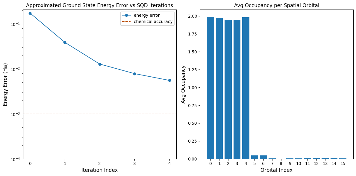
Visualize the results

The first plot shows that after a couple of iterations we estimate the ground state energy within ~6 mH (chemical accuracy is typically accepted to be 1 kcal/mol $\approx$ 1.6 mH). The energy can be improved by allowing more iterations of configuration recovery or increasing the number of samples per batch.

The second plot shows the average occupancy of each spatial orbital after the final iteration. We can see that both the spin-up and spin-down electrons occupy the first five orbitals with high probability in our solutions.

# Data for energies plot
x1 = range(len(result_history))
min_e = [
    min(result, key=lambda res: res.energy).energy + nuclear_repulsion_energy
    for result in result_history
]
e_diff = [abs(e - exact_energy) for e in min_e]
yt1 = [1.0, 1e-1, 1e-2, 1e-3, 1e-4]
 
# Chemical accuracy (+/- 1 milli-Hartree)
chem_accuracy = 0.001
 
# Data for avg spatial orbital occupancy
y2 = np.sum(result.orbital_occupancies, axis=0)
x2 = range(len(y2))
 
fig, axs = plt.subplots(1, 2, figsize=(12, 6))
 
# Plot energies
axs[0].plot(x1, e_diff, label="energy error", marker="o")
axs[0].set_xticks(x1)
axs[0].set_xticklabels(x1)
axs[0].set_yticks(yt1)
axs[0].set_yticklabels(yt1)
axs[0].set_yscale("log")
axs[0].set_ylim(1e-4)
axs[0].axhline(
    y=chem_accuracy,
    color="#BF5700",
    linestyle="--",
    label="chemical accuracy",
)
axs[0].set_title("Approximated Ground State Energy Error vs SQD Iterations")
axs[0].set_xlabel("Iteration Index", fontdict={"fontsize": 12})
axs[0].set_ylabel("Energy Error (Ha)", fontdict={"fontsize": 12})
axs[0].legend()
 
# Plot orbital occupancy
axs[1].bar(x2, y2, width=0.8)
axs[1].set_xticks(x2)
axs[1].set_xticklabels(x2)
axs[1].set_title("Avg Occupancy per Spatial Orbital")
axs[1].set_xlabel("Orbital Index", fontdict={"fontsize": 12})
axs[1].set_ylabel("Avg Occupancy", fontdict={"fontsize": 12})
 
plt.tight_layout()
plt.show()

Output:

Tutorial survey

Please take one minute to provide feedback on this tutorial. Your insights will help us improve our content offerings and user experience.

Link to survey