Krylov quantum diagonalization of lattice Hamiltonians

Usage estimate: 20 minutes on IBM Fez (NOTE: This is an estimate only. Your runtime may vary.)

Background

This tutorial demonstrates how to implement the Krylov Quantum Diagonalization Algorithm (KQD) within the context of Qiskit patterns. You will first learn about the theory behind the algorithm and then see a demonstration of its execution on a QPU.

Across disciplines, we're interested in learning ground state properties of quantum systems. Examples include understanding the fundamental nature of particles and forces, predicting and understanding the behavior of complex materials and understanding bio-chemical interactions and reactions. Because of the exponential growth of the Hilbert space and the correlation that arise in entangled systems, classical algorithm struggle to solve this problem for quantum systems of increasing size. At one end of the spectrum, existing approach that take advantage of the quantum hardware focus on variational quantum methods (e.g., variational quantum eigen-solver). These techniques face challenges with current devices because of the high number of function calls required in the optimization process, which adds a large overhead in resources once advanced error mitigation techniques are introduced, thus limiting their efficacy to small systems. At the other end of the spectrum, there are fault-tolerant quantum methods with performance guarantees (e.g., quantum phase estimation) which require deep circuits that can be executed only on a fault-tolerant device. For these reasons, we introduce here a quantum algorithm based on subspace methods (as described in this review paper), the Krylov quantum diagonalization (KQD) algorithm. This algorithm performs well at large scale [1] on existing quantum hardware, shares similar performance guarantees as phase estimation, is compatible with advanced error mitigation techniques and could provide results that are classically inaccessible.

Requirements

Before starting this tutorial, be sure you have the following installed:

• Qiskit SDK v1.0 or later, with visualization support ( pip install 'qiskit[visualization]' )
• Qiskit Runtime 0.22 or later ( pip install qiskit-ibm-runtime )

Setup

import numpy as np
import scipy as sp
import matplotlib.pylab as plt
from typing import Union, List
import itertools as it
import copy
from sympy import Matrix
import warnings
 
warnings.filterwarnings("ignore")
 
from qiskit.quantum_info import SparsePauliOp, Pauli, StabilizerState
from qiskit.circuit import Parameter
from qiskit import QuantumCircuit, QuantumRegister
from qiskit.circuit.library import PauliEvolutionGate
from qiskit.synthesis import LieTrotter
from qiskit.transpiler import Target, CouplingMap
from qiskit.transpiler.preset_passmanagers import generate_preset_pass_manager
 
 
from qiskit_ibm_runtime import (
    QiskitRuntimeService,
    EstimatorOptions,
    EstimatorV2 as Estimator,
)
 
 
def solve_regularized_gen_eig(
    h: np.ndarray,
    s: np.ndarray,
    threshold: float,
    k: int = 1,
    return_dimn: bool = False,
) -> Union[float, List[float]]:
    """
    Method for solving the generalized eigenvalue problem with regularization
 
    Args:
        h (numpy.ndarray):
            The effective representation of the matrix in the Krylov subspace
        s (numpy.ndarray):
            The matrix of overlaps between vectors of the Krylov subspace
        threshold (float):
            Cut-off value for the eigenvalue of s
        k (int):
            Number of eigenvalues to return
        return_dimn (bool):
            Whether to return the size of the regularized subspace
 
    Returns:
        lowest k-eigenvalue(s) that are the solution of the regularized generalized eigenvalue problem
 
 
    """
    s_vals, s_vecs = sp.linalg.eigh(s)
    s_vecs = s_vecs.T
    good_vecs = np.array(
        [vec for val, vec in zip(s_vals, s_vecs) if val > threshold]
    )
    h_reg = good_vecs.conj() @ h @ good_vecs.T
    s_reg = good_vecs.conj() @ s @ good_vecs.T
    if k == 1:
        if return_dimn:
            return sp.linalg.eigh(h_reg, s_reg)[0][0], len(good_vecs)
        else:
            return sp.linalg.eigh(h_reg, s_reg)[0][0]
    else:
        if return_dimn:
            return sp.linalg.eigh(h_reg, s_reg)[0][:k], len(good_vecs)
        else:
            return sp.linalg.eigh(h_reg, s_reg)[0][:k]
 
 
def single_particle_gs(H_op, n_qubits):
    """
    Find the ground state of the single particle(excitation) sector
    """
    H_x = []
    for p, coeff in H_op.to_list():
        H_x.append(set([i for i, v in enumerate(Pauli(p).x) if v]))
 
    H_z = []
    for p, coeff in H_op.to_list():
        H_z.append(set([i for i, v in enumerate(Pauli(p).z) if v]))
 
    H_c = H_op.coeffs
 
    print("n_sys_qubits", n_qubits)
 
    n_exc = 1
    sub_dimn = int(sp.special.comb(n_qubits + 1, n_exc))
    print("n_exc", n_exc, ", subspace dimension", sub_dimn)
 
    few_particle_H = np.zeros((sub_dimn, sub_dimn), dtype=complex)
 
    sparse_vecs = [
        set(vec) for vec in it.combinations(range(n_qubits + 1), r=n_exc)
    ]  # list all of the possible sets of n_exc indices of 1s in n_exc-particle states
 
    m = 0
    for i, i_set in enumerate(sparse_vecs):
        for j, j_set in enumerate(sparse_vecs):
            m += 1
 
            if len(i_set.symmetric_difference(j_set)) <= 2:
                for p_x, p_z, coeff in zip(H_x, H_z, H_c):
                    if i_set.symmetric_difference(j_set) == p_x:
                        sgn = ((-1j) ** len(p_x.intersection(p_z))) * (
                            (-1) ** len(i_set.intersection(p_z))
                        )
                    else:
                        sgn = 0
 
                    few_particle_H[i, j] += sgn * coeff
 
    gs_en = min(np.linalg.eigvalsh(few_particle_H))
    print("single particle ground state energy: ", gs_en)
    return gs_en

Step 1: Map classical inputs to a quantum problem

The Krylov space

The Krylov space $\mathcal{K}^r$ of order $r$ is the space spanned by vectors obtained by multiplying higher powers of a matrix $A$, up to $r-1$, with a reference vector $\vert v \rangle$.

If the matrix $A$ is the Hamiltonian $H$, we'll refer to the corresponding space as the power Krylov space $\mathcal{K}_P$. In the case where $A$ is the time-evolution operator generated by the Hamiltonian $U=e^{-iHt}$, we'll refer to the space as the unitary Krylov space $\mathcal{K}_U$. The power Krylov subspace that we use classically cannot be generated directly on a quantum computer as $H$ is not a unitary operator. Instead, we can use the time-evolution operator $U = e^{-iHt}$ which can be shown to give similar convergence guarantees as the power method. Powers of $U$ then become different time steps $U^k = e^{-iH(kt)}$.

See the Appendix for a detailed derivation of how the unitary Krylov space allows to represents low-energy eigenstates accurately.

Krylov quantum diagonalization algorithm

Given an Hamiltonian $H$ that we wish to diagonalize, first we consider the corresponding unitary Krylov space $\mathcal{K}_U$. The goal is to find a compact representation of the Hamiltonian in $\mathcal{K}_U$, which we'll refer to as $\tilde{H}$. The matrix elements of $\tilde{H}$, the projection of the Hamiltonian in the Krylov space, can be calculated by calculating the following expectation values

Where $\vert \psi_n \rangle = e^{-i H t_n} \vert \psi \rangle$ are the vectors of the unitary Krylov space and $t_n = n dt$ are the multiples of the time step $dt$ chosen. On a quantum computer, the calculation of each matrix elements can be done with any algorithm which allows to obtain overlap between quantum states. In this tutorial we'll focus on the Hadamard test. Given that the $\mathcal{K}_U$ has dimension $r$, the Hamiltonian projected into the subspace will have dimensions $r \times r$. With $r$ small enough (generally $r<<100$ is sufficient to obtain convergence of estimates of eigenenergies) we can then easily diagonalize the projected Hamiltonian $\tilde{H}$. However, we cannot directly diagonalize $\tilde{H}$ because of the non-orthogonality of the Krylov space vectors. We'll have to measure their overlaps and construct a matrix $\tilde{S}$

This allows us to solve the eigenvalue problem in a non-orthogonal space (also called generalized eigenvalue problem)

One can then obtain estimates of the eigenvalues and eigenstates of $H$ by looking at the ones of $\tilde{H}$. For example, the estimate of the ground state energy is obtained by taking the smallest eigenvalue $c$ and the ground state from the corresponding eigenvector $\vec{c}$. The coefficients in $\vec{c}$ determines the contribution of the different vectors that span $\mathcal{K}_U$.

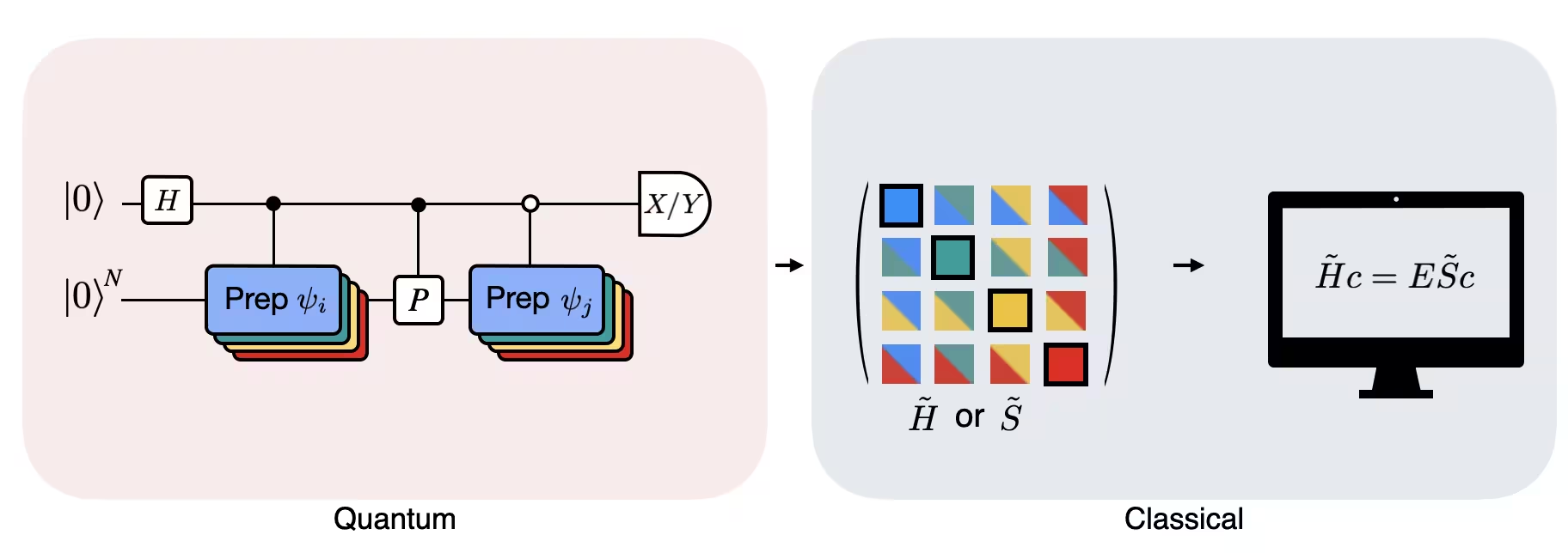
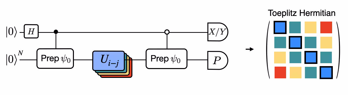
The Figure shows a circuit representation of the modified Hadamard test, a method that is used to compute the overlap between different quantum states. For each matrix element $\tilde{H}_{i,j}$, a Hadamard test between the state $\vert \psi_i \rangle$, $\vert \psi_j \rangle$ is carried out. This is highlighted in the figure by the color scheme for the matrix elements and the corresponding $\text{Prep} \; \psi_i$, $\text{Prep} \; \psi_j$ operations. Thus, a set of Hadamard tests for all the possible combinations of Krylov space vectors is required to compute all the matrix elements of the projected Hamiltonian $\tilde{H}$. The top wire in the Hadamard test circuit is an ancilla qubit which is measured either in the X or Y basis, its expectation value determines the value of the overlap between the states. The bottom wire represents all the qubits of the system Hamiltonian. The $\text{Prep} \; \psi_i$ operation prepares the system qubit in the state $\vert \psi_i \rangle$ controlled by the state of the ancilla qubit (similarly for $\text{Prep} \; \psi_j$) and the operation $P$ represents Pauli decomposition of the system Hamiltonian $H = \sum_i P_i$. A more detailed derivation of the operations calculated by the Hadamard test is given below.

Define Hamiltonian

Let's consider the Heisenberg Hamiltonian for $N$ qubits on a linear chain: $H= \sum_{i,j}^N X_i X_j + Y_i Y_j - J Z_i Z_j$

# Define problem Hamiltonian.
n_qubits = 30
J = 1  # coupling strength for ZZ interaction
 
# Define the Hamiltonian:
H_int = [["I"] * n_qubits for _ in range(3 * (n_qubits - 1))]
for i in range(n_qubits - 1):
    H_int[i][i] = "Z"
    H_int[i][i + 1] = "Z"
for i in range(n_qubits - 1):
    H_int[n_qubits - 1 + i][i] = "X"
    H_int[n_qubits - 1 + i][i + 1] = "X"
for i in range(n_qubits - 1):
    H_int[2 * (n_qubits - 1) + i][i] = "Y"
    H_int[2 * (n_qubits - 1) + i][i + 1] = "Y"
H_int = ["".join(term) for term in H_int]
H_tot = [(term, J) if term.count("Z") == 2 else (term, 1) for term in H_int]
 
# Get operator
H_op = SparsePauliOp.from_list(H_tot)
print(H_tot)

Output:

[('ZZIIIIIIIIIIIIIIIIIIIIIIIIIIII', 1), ('IZZIIIIIIIIIIIIIIIIIIIIIIIIIII', 1), ('IIZZIIIIIIIIIIIIIIIIIIIIIIIIII', 1), ('IIIZZIIIIIIIIIIIIIIIIIIIIIIIII', 1), ('IIIIZZIIIIIIIIIIIIIIIIIIIIIIII', 1), ('IIIIIZZIIIIIIIIIIIIIIIIIIIIIII', 1), ('IIIIIIZZIIIIIIIIIIIIIIIIIIIIII', 1), ('IIIIIIIZZIIIIIIIIIIIIIIIIIIIII', 1), ('IIIIIIIIZZIIIIIIIIIIIIIIIIIIII', 1), ('IIIIIIIIIZZIIIIIIIIIIIIIIIIIII', 1), ('IIIIIIIIIIZZIIIIIIIIIIIIIIIIII', 1), ('IIIIIIIIIIIZZIIIIIIIIIIIIIIIII', 1), ('IIIIIIIIIIIIZZIIIIIIIIIIIIIIII', 1), ('IIIIIIIIIIIIIZZIIIIIIIIIIIIIII', 1), ('IIIIIIIIIIIIIIZZIIIIIIIIIIIIII', 1), ('IIIIIIIIIIIIIIIZZIIIIIIIIIIIII', 1), ('IIIIIIIIIIIIIIIIZZIIIIIIIIIIII', 1), ('IIIIIIIIIIIIIIIIIZZIIIIIIIIIII', 1), ('IIIIIIIIIIIIIIIIIIZZIIIIIIIIII', 1), ('IIIIIIIIIIIIIIIIIIIZZIIIIIIIII', 1), ('IIIIIIIIIIIIIIIIIIIIZZIIIIIIII', 1), ('IIIIIIIIIIIIIIIIIIIIIZZIIIIIII', 1), ('IIIIIIIIIIIIIIIIIIIIIIZZIIIIII', 1), ('IIIIIIIIIIIIIIIIIIIIIIIZZIIIII', 1), ('IIIIIIIIIIIIIIIIIIIIIIIIZZIIII', 1), ('IIIIIIIIIIIIIIIIIIIIIIIIIZZIII', 1), ('IIIIIIIIIIIIIIIIIIIIIIIIIIZZII', 1), ('IIIIIIIIIIIIIIIIIIIIIIIIIIIZZI', 1), ('IIIIIIIIIIIIIIIIIIIIIIIIIIIIZZ', 1), ('XXIIIIIIIIIIIIIIIIIIIIIIIIIIII', 1), ('IXXIIIIIIIIIIIIIIIIIIIIIIIIIII', 1), ('IIXXIIIIIIIIIIIIIIIIIIIIIIIIII', 1), ('IIIXXIIIIIIIIIIIIIIIIIIIIIIIII', 1), ('IIIIXXIIIIIIIIIIIIIIIIIIIIIIII', 1), ('IIIIIXXIIIIIIIIIIIIIIIIIIIIIII', 1), ('IIIIIIXXIIIIIIIIIIIIIIIIIIIIII', 1), ('IIIIIIIXXIIIIIIIIIIIIIIIIIIIII', 1), ('IIIIIIIIXXIIIIIIIIIIIIIIIIIIII', 1), ('IIIIIIIIIXXIIIIIIIIIIIIIIIIIII', 1), ('IIIIIIIIIIXXIIIIIIIIIIIIIIIIII', 1), ('IIIIIIIIIIIXXIIIIIIIIIIIIIIIII', 1), ('IIIIIIIIIIIIXXIIIIIIIIIIIIIIII', 1), ('IIIIIIIIIIIIIXXIIIIIIIIIIIIIII', 1), ('IIIIIIIIIIIIIIXXIIIIIIIIIIIIII', 1), ('IIIIIIIIIIIIIIIXXIIIIIIIIIIIII', 1), ('IIIIIIIIIIIIIIIIXXIIIIIIIIIIII', 1), ('IIIIIIIIIIIIIIIIIXXIIIIIIIIIII', 1), ('IIIIIIIIIIIIIIIIIIXXIIIIIIIIII', 1), ('IIIIIIIIIIIIIIIIIIIXXIIIIIIIII', 1), ('IIIIIIIIIIIIIIIIIIIIXXIIIIIIII', 1), ('IIIIIIIIIIIIIIIIIIIIIXXIIIIIII', 1), ('IIIIIIIIIIIIIIIIIIIIIIXXIIIIII', 1), ('IIIIIIIIIIIIIIIIIIIIIIIXXIIIII', 1), ('IIIIIIIIIIIIIIIIIIIIIIIIXXIIII', 1), ('IIIIIIIIIIIIIIIIIIIIIIIIIXXIII', 1), ('IIIIIIIIIIIIIIIIIIIIIIIIIIXXII', 1), ('IIIIIIIIIIIIIIIIIIIIIIIIIIIXXI', 1), ('IIIIIIIIIIIIIIIIIIIIIIIIIIIIXX', 1), ('YYIIIIIIIIIIIIIIIIIIIIIIIIIIII', 1), ('IYYIIIIIIIIIIIIIIIIIIIIIIIIIII', 1), ('IIYYIIIIIIIIIIIIIIIIIIIIIIIIII', 1), ('IIIYYIIIIIIIIIIIIIIIIIIIIIIIII', 1), ('IIIIYYIIIIIIIIIIIIIIIIIIIIIIII', 1), ('IIIIIYYIIIIIIIIIIIIIIIIIIIIIII', 1), ('IIIIIIYYIIIIIIIIIIIIIIIIIIIIII', 1), ('IIIIIIIYYIIIIIIIIIIIIIIIIIIIII', 1), ('IIIIIIIIYYIIIIIIIIIIIIIIIIIIII', 1), ('IIIIIIIIIYYIIIIIIIIIIIIIIIIIII', 1), ('IIIIIIIIIIYYIIIIIIIIIIIIIIIIII', 1), ('IIIIIIIIIIIYYIIIIIIIIIIIIIIIII', 1), ('IIIIIIIIIIIIYYIIIIIIIIIIIIIIII', 1), ('IIIIIIIIIIIIIYYIIIIIIIIIIIIIII', 1), ('IIIIIIIIIIIIIIYYIIIIIIIIIIIIII', 1), ('IIIIIIIIIIIIIIIYYIIIIIIIIIIIII', 1), ('IIIIIIIIIIIIIIIIYYIIIIIIIIIIII', 1), ('IIIIIIIIIIIIIIIIIYYIIIIIIIIIII', 1), ('IIIIIIIIIIIIIIIIIIYYIIIIIIIIII', 1), ('IIIIIIIIIIIIIIIIIIIYYIIIIIIIII', 1), ('IIIIIIIIIIIIIIIIIIIIYYIIIIIIII', 1), ('IIIIIIIIIIIIIIIIIIIIIYYIIIIIII', 1), ('IIIIIIIIIIIIIIIIIIIIIIYYIIIIII', 1), ('IIIIIIIIIIIIIIIIIIIIIIIYYIIIII', 1), ('IIIIIIIIIIIIIIIIIIIIIIIIYYIIII', 1), ('IIIIIIIIIIIIIIIIIIIIIIIIIYYIII', 1), ('IIIIIIIIIIIIIIIIIIIIIIIIIIYYII', 1), ('IIIIIIIIIIIIIIIIIIIIIIIIIIIYYI', 1), ('IIIIIIIIIIIIIIIIIIIIIIIIIIIIYY', 1)]

Set parameters for the algorithm

We heuristically choose a value for the time-step dt (based on upper bounds on the Hamiltonian norm). Ref [2] showed that a sufficiently small timestep is $\pi/\vert \vert H \vert \vert$, and that it is preferable up to a point to underestimate this value rather than overestimate, since overestimating can allow contributions from high-energy states to corrupt even the optimal state in the Krylov space. On the other hand, choosing $dt$ to be too small leads to worse conditioning of the Krylov subspace, since the Krylov basis vectors differ less from timestep to timestep.

# Get Hamiltonian restricted to single-particle states
single_particle_H = np.zeros((n_qubits, n_qubits))
for i in range(n_qubits):
    for j in range(i + 1):
        for p, coeff in H_op.to_list():
            p_x = Pauli(p).x
            p_z = Pauli(p).z
            if all(
                p_x[k] == ((i == k) + (j == k)) % 2 for k in range(n_qubits)
            ):
                sgn = (
                    (-1j) ** sum(p_z[k] and p_x[k] for k in range(n_qubits))
                ) * ((-1) ** p_z[i])
            else:
                sgn = 0
            single_particle_H[i, j] += sgn * coeff
for i in range(n_qubits):
    for j in range(i + 1, n_qubits):
        single_particle_H[i, j] = np.conj(single_particle_H[j, i])
 
# Set dt according to spectral norm
dt = np.pi / np.linalg.norm(single_particle_H, ord=2)
dt

Output:

0.10833078115826872

And set other parameters of the algorithm. For the sake of this tutorial, we'll limit ourselves to using a Krylov space with only 5 dimensions, which is quite limiting.

# Set parameters for quantum Krylov algorithm
krylov_dim = 5  # size of Krylov subspace
num_trotter_steps = 6
dt_circ = dt / num_trotter_steps

State preparation

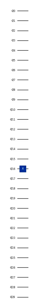
Pick a reference state $\vert \psi \rangle$ that has some overlap with the ground state. For this Hamiltonian, We use the a state with an excitation in the middle qubit $\vert 00..010...00 \rangle$ as our reference state.

qc_state_prep = QuantumCircuit(n_qubits)
qc_state_prep.x(int(n_qubits / 2) + 1)
qc_state_prep.draw("mpl", scale=0.5)

Output:

Time evolution

We can realize the time-evolution operator generated by a given Hamiltonian: $U=e^{-iHt}$ via the Lie-Trotter approximation.

t = Parameter("t")
 
## Create the time-evo op circuit
evol_gate = PauliEvolutionGate(
    H_op, time=t, synthesis=LieTrotter(reps=num_trotter_steps)
)
 
qr = QuantumRegister(n_qubits)
qc_evol = QuantumCircuit(qr)
qc_evol.append(evol_gate, qargs=qr)

Output:

<qiskit.circuit.instructionset.InstructionSet at 0x136639060>

Hadamard test

Where $P$ is one of the terms in the decomposition of the Hamiltonian $H=\sum P$ and $\text{Prep} \; \psi_i$, $\text{Prep} \; \psi_j$ are controlled operations that prepare $|\psi_i\rangle$, $|\psi_j\rangle$ vectors of the unitary Krylov space, with $|\psi_k\rangle = e^{-i H k dt } \vert \psi \rangle = e^{-i H k dt } U_{\psi} \vert 0 \rangle^N$. To measure $X$, first apply $H$...

... then measure:

From the identity $|a + b\|^2 = \langle a + b | a + b \rangle = \|a\|^2 + \|b\|^2 + 2\text{Re}\langle a | b \rangle$. Similarly, measuring $Y$ yields

## Create the time-evo op circuit
evol_gate = PauliEvolutionGate(
    H_op, time=dt, synthesis=LieTrotter(reps=num_trotter_steps)
)
 
## Create the time-evo op dagger circuit
evol_gate_d = PauliEvolutionGate(
    H_op, time=dt, synthesis=LieTrotter(reps=num_trotter_steps)
)
evol_gate_d = evol_gate_d.inverse()
 
# Put pieces together
qc_reg = QuantumRegister(n_qubits)
qc_temp = QuantumCircuit(qc_reg)
qc_temp.compose(qc_state_prep, inplace=True)
for _ in range(num_trotter_steps):
    qc_temp.append(evol_gate, qargs=qc_reg)
for _ in range(num_trotter_steps):
    qc_temp.append(evol_gate_d, qargs=qc_reg)
qc_temp.compose(qc_state_prep.inverse(), inplace=True)
 
# Create controlled version of the circuit
controlled_U = qc_temp.to_gate().control(1)
 
# Create hadamard test circuit for real part
qr = QuantumRegister(n_qubits + 1)
qc_real = QuantumCircuit(qr)
qc_real.h(0)
qc_real.append(controlled_U, list(range(n_qubits + 1)))
qc_real.h(0)
 
print(
    "Circuit for calculating the real part of the overlap in S via Hadamard test"
)
qc_real.draw("mpl", fold=-1, scale=0.5)

Output:

Circuit for calculating the real part of the overlap in S via Hadamard test

The Hadamard test circuit can be a deep circuit once we decompose to native gates (which will increase even more if we account for the topology of the device)

print(
    "Number of layers of 2Q operations",
    qc_real.decompose(reps=2).depth(lambda x: x[0].num_qubits == 2),
)

Output:

Number of layers of 2Q operations 120003

Step 2: Optimize problem for quantum hardware execution

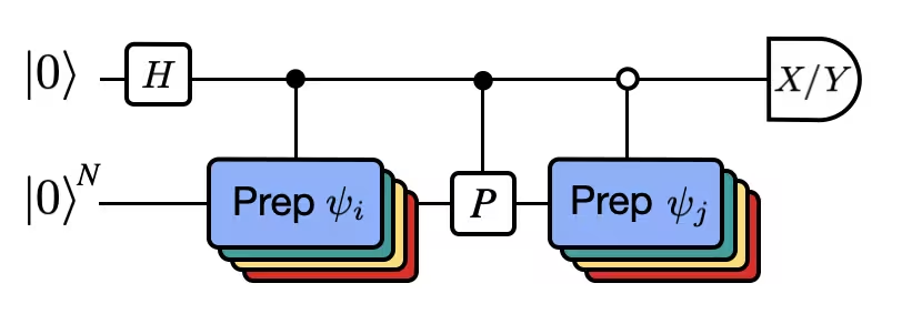
Efficient Hadamard test

We can optimize the deep circuits for the Hadamard test that we have obtained by introducing some approximations and relying on some assumption about the model Hamiltonian. For example, consider the following circuit for the Hadamard test:

Assume we can classically calculate $E_0$, the eigenvalue of $|0\rangle^N$ under the Hamiltonian $H$. This is satisfied when the Hamiltonian preserves the U(1) symmetry. Although this may seem like a strong assumption, there are many cases where it is safe to assume that there is a vacuum state (in this case it maps to the $|0\rangle^N$ state) which is unaffected by the action of the Hamiltonian. This is true for example for chemistry Hamiltonians that describe stable molecule (where the number of electrons is conserved). Given that the gate $\text{Prep} \; \psi$, prepares the desired reference state $\ket{psi} = \text{Prep} \; \psi \ket{0} = e^{-i H 0 dt} U_{\psi} \ket{0}$, e.g., to prepare the HF state for chemistry $\text{Prep} \; \psi$ would be a product of single-qubit NOTs, so controlled-$\text{Prep} \; \psi$ is just a product of CNOTs. Then the circuit above implements the following state prior to measurement:

where we have used the classical simulable phase shift $U\ket{0}^N = e^{i\phi}\ket{0}^N$ in the third line. Therefore the expectation values are obtained as

Using these assumptions we were able to write the expectation values of operators of interest with fewer controlled operations. In fact, we only need to implement the controlled state preparation $\text{Prep} \; \psi$ and not controlled time evolutions. Reframing our calculation as above will allow us to greatly reduce the depth of the resulting circuits.

Decompose time-evolution operator with Trotter decomposition

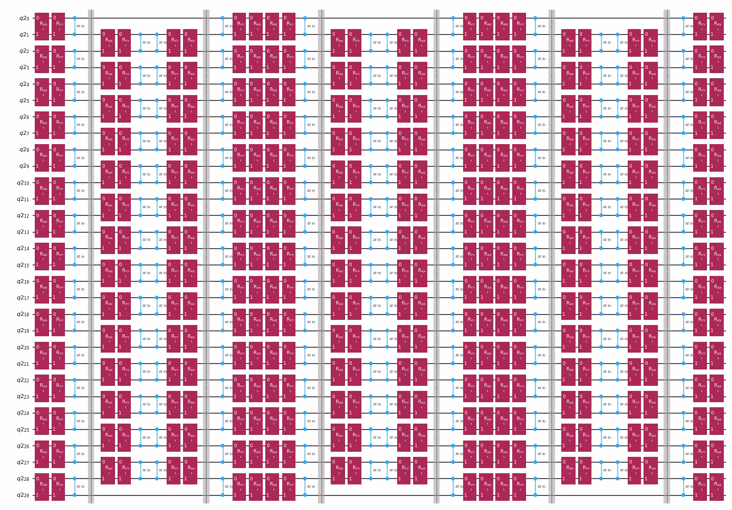
Instead of implementing the time-evolution operator exactly we can use the Trotter decomposition to implement an approximation of it. Repeating several times a certain order Trotter decomposition gives us further reduction of the error introduced from the approximation. In the following, we directly build the Trotter implementation in the most efficient way for the interaction graph of the Hamiltonian we are considering (nearest neighbor interactions only). In practice we insert Pauli rotations $R_{xx}$, $R_{yy}$, $R_{zz}$ with a parametrized angle $t$ which correspond to the approximate implementation of $e^{-i (XX + YY + ZZ) t}$. Given the difference in definition of the Pauli rotations and the time-evolution that we are trying to implement, we'll have to use the parameter $2*dt$ to achieve a time-evolution of $dt$. Furthermore, we reverse the order of the operations for odd number of repetitions of the Trotter steps, which is functionally equivalent but allows for synthesizing adjacent operations in a single $SU(2)$ unitary. This gives a much shallower circuit than what is obtained using the generic PauliEvolutionGate() functionality.

t = Parameter("t")
 
# Create instruction for rotation about XX+YY-ZZ:
Rxyz_circ = QuantumCircuit(2)
Rxyz_circ.rxx(t, 0, 1)
Rxyz_circ.ryy(t, 0, 1)
Rxyz_circ.rzz(t, 0, 1)
Rxyz_instr = Rxyz_circ.to_instruction(label="RXX+YY+ZZ")
 
interaction_list = [
    [[i, i + 1] for i in range(0, n_qubits - 1, 2)],
    [[i, i + 1] for i in range(1, n_qubits - 1, 2)],
]  # linear chain
 
qr = QuantumRegister(n_qubits)
trotter_step_circ = QuantumCircuit(qr)
for i, color in enumerate(interaction_list):
    for interaction in color:
        trotter_step_circ.append(Rxyz_instr, interaction)
    if i < len(interaction_list) - 1:
        trotter_step_circ.barrier()
reverse_trotter_step_circ = trotter_step_circ.reverse_ops()
 
qc_evol = QuantumCircuit(qr)
for step in range(num_trotter_steps):
    if step % 2 == 0:
        qc_evol = qc_evol.compose(trotter_step_circ)
    else:
        qc_evol = qc_evol.compose(reverse_trotter_step_circ)
 
qc_evol.decompose().draw("mpl", fold=-1, scale=0.5)

Output:

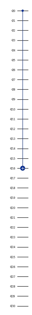
Use an optimized circuit for state preparation

control = 0
excitation = int(n_qubits / 2) + 1
controlled_state_prep = QuantumCircuit(n_qubits + 1)
controlled_state_prep.cx(control, excitation)
controlled_state_prep.draw("mpl", fold=-1, scale=0.5)

Output:

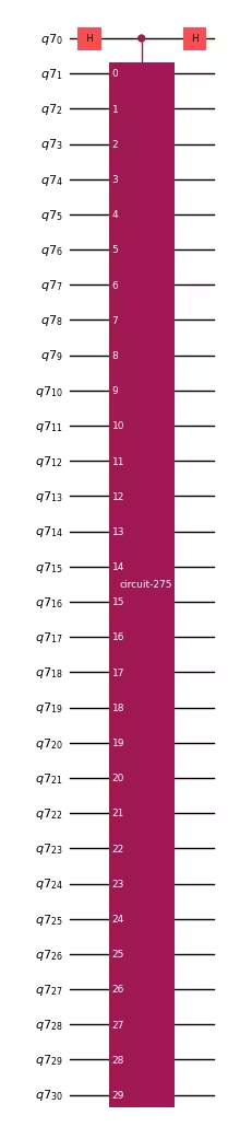
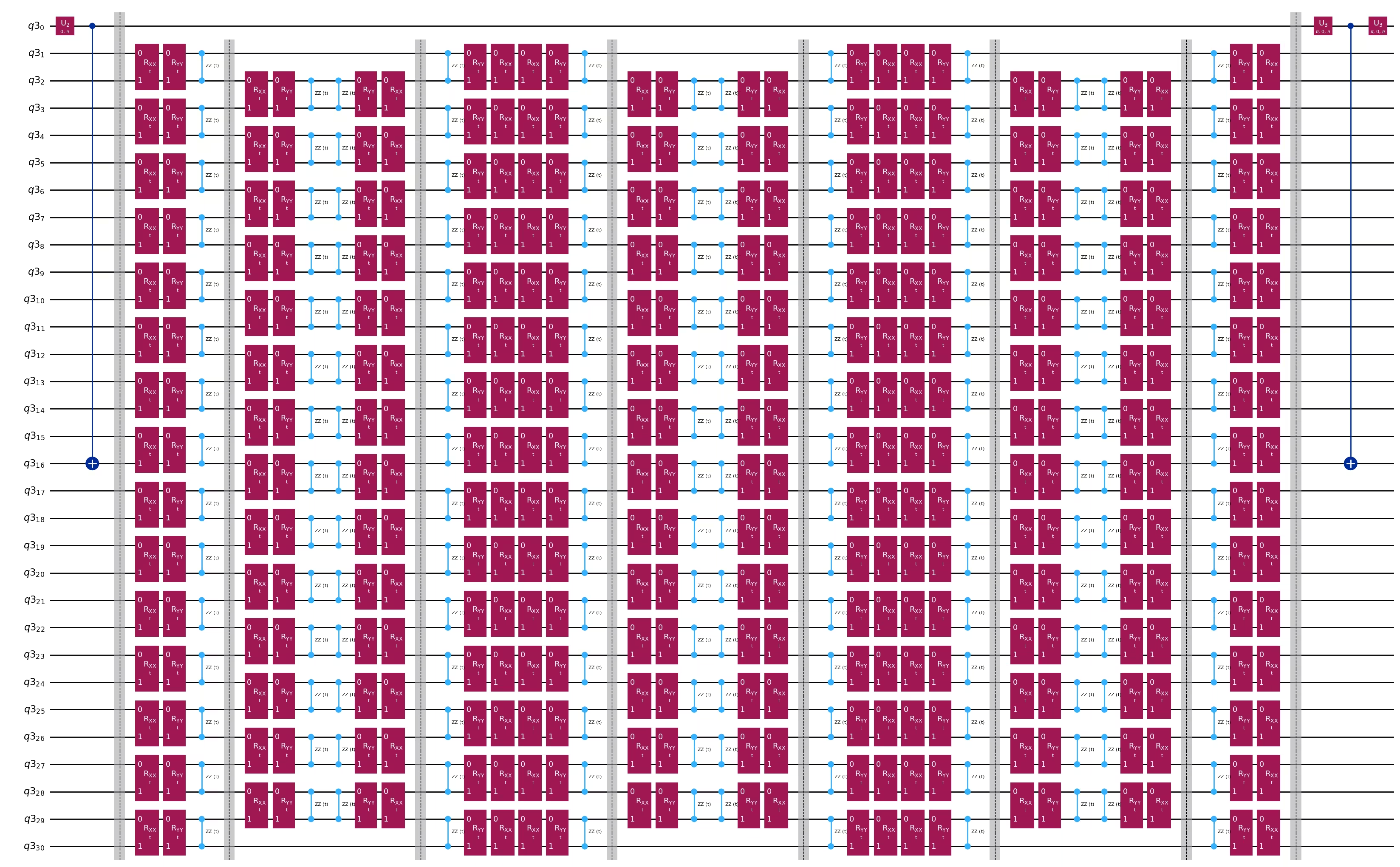
Template circuits for calculating matrix elements of $\tilde{S}$ and $\tilde{H}$ via Hadamard test

The only difference between the circuits used in the Hadamard test will be the phase in the time-evolution operator and the observables measured. Therefore we can prepare a template circuit which represent the generic circuit for the Hadamard test, with placeholders for the gates that depend on the time-evolution operator.

# Parameters for the template circuits
parameters = []
for idx in range(1, krylov_dim):
    parameters.append(2 * dt_circ * (idx))

# Create modified hadamard test circuit
qr = QuantumRegister(n_qubits + 1)
qc = QuantumCircuit(qr)
qc.h(0)
qc.compose(controlled_state_prep, list(range(n_qubits + 1)), inplace=True)
qc.barrier()
qc.compose(qc_evol, list(range(1, n_qubits + 1)), inplace=True)
qc.barrier()
qc.x(0)
qc.compose(
    controlled_state_prep.inverse(), list(range(n_qubits + 1)), inplace=True
)
qc.x(0)
 
qc.decompose().draw("mpl", fold=-1)

Output:

print(
    "The optimized circuit has 2Q gates depth: ",
    qc.decompose().decompose().depth(lambda x: x[0].num_qubits == 2),
)

Output:

The optimized circuit has 2Q gates depth:  74

We have considerably reduced the depth of the Hadamard test with a combination of Trotter approximation and uncontrolled unitaries

Step 3: Execute using Qiskit primitives

Instantiate the backend and set runtime parameters

service = QiskitRuntimeService()
backend = service.least_busy(
    operational=True, simulator=False, min_num_qubits=127
)

Transpiling to a QPU

First, let's pick subsets of the coupling map with "good" performing qubits (where "good" is pretty arbitraty here, we mostly want to avoid really poor performing qubits) and create a new target for transpilation

target = backend.target
cmap = target.build_coupling_map(filter_idle_qubits=True)
cmap_list = list(cmap.get_edges())
 
cust_cmap_list = copy.deepcopy(cmap_list)
for q in range(target.num_qubits):
    meas_err = target["measure"][(q,)].error
    t2 = target.qubit_properties[q].t2 * 1e6
    if meas_err > 0.05 or t2 < 30:
        # print(q)
        for q_pair in cmap_list:
            if q in q_pair:
                try:
                    cust_cmap_list.remove(q_pair)
                except:
                    continue
 
for q in cmap_list:
    twoq_gate_err = target["cz"][q].error
    if twoq_gate_err > 0.015:
        for q_pair in cmap_list:
            if q == q_pair:
                try:
                    cust_cmap_list.remove(q)
                except:
                    continue
 
 
cust_cmap = CouplingMap(cust_cmap_list)
cust_target = Target.from_configuration(
    basis_gates=backend.configuration().basis_gates,
    coupling_map=cust_cmap,
)

Then transpile the virtual circuit to the best physical layout in this new target

basis_gates = list(target.operation_names)
pm = generate_preset_pass_manager(
    optimization_level=3,
    target=cust_target,
    basis_gates=basis_gates,
)
 
qc_trans = pm.run(qc)
 
print("depth", qc_trans.depth(lambda x: x[0].num_qubits == 2))
print("num 2q ops", qc_trans.count_ops())
print(
    "physical qubits",
    sorted(
        [
            idx
            for idx, qb in qc_trans.layout.initial_layout.get_physical_bits().items()
            if qb._register.name != "ancilla"
        ]
    ),
)

Create PUBs for execution with Estimator

# Define observables to measure for S
observable_S_real = "I" * (n_qubits) + "X"
observable_S_imag = "I" * (n_qubits) + "Y"
 
observable_op_real = SparsePauliOp(
    observable_S_real
)  # define a sparse pauli operator for the observable
observable_op_imag = SparsePauliOp(observable_S_imag)
 
layout = qc_trans.layout  # get layout of transpiled circuit
observable_op_real = observable_op_real.apply_layout(
    layout
)  # apply physical layout to the observable
observable_op_imag = observable_op_imag.apply_layout(layout)
observable_S_real = (
    observable_op_real.paulis.to_labels()
)  # get the label of the physical observable
observable_S_imag = observable_op_imag.paulis.to_labels()
 
observables_S = [[observable_S_real], [observable_S_imag]]
 
 
# Define observables to measure for H
# Hamiltonian terms to measure
observable_list = []
for pauli, coeff in zip(H_op.paulis, H_op.coeffs):
    # print(pauli)
    observable_H_real = pauli[::-1].to_label() + "X"
    observable_H_imag = pauli[::-1].to_label() + "Y"
    observable_list.append([observable_H_real])
    observable_list.append([observable_H_imag])
 
layout = qc_trans.layout
 
observable_trans_list = []
for observable in observable_list:
    observable_op = SparsePauliOp(observable)
    observable_op = observable_op.apply_layout(layout)
    observable_trans_list.append([observable_op.paulis.to_labels()])
 
observables_H = observable_trans_list
 
 
# Define a sweep over parameter values
params = np.vstack(parameters).T
 
 
# Estimate the expectation value for all combinations of
# observables and parameter values, where the pub result will have
# shape (# observables, # parameter values).
pub = (qc_trans, observables_S + observables_H, params)

Run circuits

Circuits for $t=0$ are classically calculable

qc_cliff = qc.assign_parameters({t: 0})
 
 
# Get expectation values from experiment
S_expval_real = StabilizerState(qc_cliff).expectation_value(
    Pauli("I" * (n_qubits) + "X")
)
S_expval_imag = StabilizerState(qc_cliff).expectation_value(
    Pauli("I" * (n_qubits) + "Y")
)
 
# Get expectation values
S_expval = S_expval_real + 1j * S_expval_imag
 
H_expval = 0
for obs_idx, (pauli, coeff) in enumerate(zip(H_op.paulis, H_op.coeffs)):
    # Get expectation values from experiment
    expval_real = StabilizerState(qc_cliff).expectation_value(
        Pauli(pauli[::-1].to_label() + "X")
    )
    expval_imag = StabilizerState(qc_cliff).expectation_value(
        Pauli(pauli[::-1].to_label() + "Y")
    )
    expval = expval_real + 1j * expval_imag
 
    # Fill-in matrix elements
    H_expval += coeff * expval
 
 
print(H_expval)

Output:

(25+0j)

Execute circuits for $S$ and $\tilde{H}$ with the Estimator

# Experiment options
num_randomizations = 300
num_randomizations_learning = 30
shots_per_randomization = 100
noise_factors = [1, 1.2, 1.4]
learning_pair_depths = [0, 4, 24, 48]
 
 
experimental_opts = {}
experimental_opts["execution_path"] = "gen3-turbo"
experimental_opts["resilience"] = {
    "measure_mitigation": True,
    "measure_noise_learning": {
        "num_randomizations": num_randomizations_learning,
        "shots_per_randomization": shots_per_randomization,
    },
    "zne_mitigation": True,
    "zne": {"noise_factors": noise_factors},
    "layer_noise_learning": {
        "max_layers_to_learn": 10,
        "layer_pair_depths": learning_pair_depths,
        "shots_per_randomization": shots_per_randomization,
        "num_randomizations": num_randomizations_learning,
    },
    "zne": {
        "amplifier": "pea",
        "return_all_extrapolated": True,
        "return_unextrapolated": True,
        "extrapolated_noise_factors": [0] + noise_factors,
    },
}
experimental_opts["twirling"] = {
    "num_randomizations": num_randomizations,
    "shots_per_randomization": shots_per_randomization,
    "strategy": "all",
    # 'strategy':'active-accum'
}
 
options = EstimatorOptions(experimental=experimental_opts)
estimator = Estimator(mode=backend, options=options)
 
 
job = estimator.run([pub])

Step 4: Post-process and return result in desired classical format

results = job.result()[0]

Calculate Effective Hamiltonian and Overlap matrices

First calculate the phase accumulated by the $\vert 0 \rangle$ state during the uncontrolled time evolution

prefactors = [
    np.exp(-1j * sum([c for p, c in H_op.to_list() if "Z" in p]) * i * dt)
    for i in range(1, krylov_dim)
]

Once we have the results of the circuit executions we can post-process the data to calculate the matrix elements of $S$

# Assemble S, the overlap matrix of dimension D:
S_first_row = np.zeros(krylov_dim, dtype=complex)
S_first_row[0] = 1 + 0j
 
# Add in ancilla-only measurements:
for i in range(krylov_dim - 1):
    # Get expectation values from experiment
    expval_real = results.data.evs[0][0][
        i
    ]  # automatic extrapolated evs if ZNE is used
    expval_imag = results.data.evs[1][0][
        i
    ]  # automatic extrapolated evs if ZNE is used
 
    # Get expectation values
    expval = expval_real + 1j * expval_imag
    S_first_row[i + 1] += prefactors[i] * expval
 
S_first_row_list = S_first_row.tolist()  # for saving purposes
 
 
S_circ = np.zeros((krylov_dim, krylov_dim), dtype=complex)
 
# Distribute entries from first row across matrix:
for i, j in it.product(range(krylov_dim), repeat=2):
    if i >= j:
        S_circ[j, i] = S_first_row[i - j]
    else:
        S_circ[j, i] = np.conj(S_first_row[j - i])

Matrix(S_circ)

Output:

$\displaystyle \left[\begin{matrix}1.0 & -0.723052998582984 - 0.345085413575966 i & 0.467051960502366 + 0.516197865254034 i & -0.180546747798251 - 0.492624093654174 i & 0.0012070853532697 + 0.312052218182462 i\\-0.723052998582984 + 0.345085413575966 i & 1.0 & -0.723052998582984 - 0.345085413575966 i & 0.467051960502366 + 0.516197865254034 i & -0.180546747798251 - 0.492624093654174 i\\0.467051960502366 - 0.516197865254034 i & -0.723052998582984 + 0.345085413575966 i & 1.0 & -0.723052998582984 - 0.345085413575966 i & 0.467051960502366 + 0.516197865254034 i\\-0.180546747798251 + 0.492624093654174 i & 0.467051960502366 - 0.516197865254034 i & -0.723052998582984 + 0.345085413575966 i & 1.0 & -0.723052998582984 - 0.345085413575966 i\\0.0012070853532697 - 0.312052218182462 i & -0.180546747798251 + 0.492624093654174 i & 0.467051960502366 - 0.516197865254034 i & -0.723052998582984 + 0.345085413575966 i & 1.0\end{matrix}\right]$

And the matrix elements of $\tilde{H}$

# Assemble S, the overlap matrix of dimension D:
H_first_row = np.zeros(krylov_dim, dtype=complex)
H_first_row[0] = H_expval
 
for obs_idx, (pauli, coeff) in enumerate(zip(H_op.paulis, H_op.coeffs)):
    # Add in ancilla-only measurements:
    for i in range(krylov_dim - 1):
        # Get expectation values from experiment
        expval_real = results.data.evs[2 + 2 * obs_idx][0][
            i
        ]  # automatic extrapolated evs if ZNE is used
        expval_imag = results.data.evs[2 + 2 * obs_idx + 1][0][
            i
        ]  # automatic extrapolated evs if ZNE is used
 
        # Get expectation values
        expval = expval_real + 1j * expval_imag
        H_first_row[i + 1] += prefactors[i] * coeff * expval
 
H_first_row_list = H_first_row.tolist()
 
H_eff_circ = np.zeros((krylov_dim, krylov_dim), dtype=complex)
 
# Distribute entries from first row across matrix:
for i, j in it.product(range(krylov_dim), repeat=2):
    if i >= j:
        H_eff_circ[j, i] = H_first_row[i - j]
    else:
        H_eff_circ[j, i] = np.conj(H_first_row[j - i])

Matrix(H_eff_circ)

Output:

$\displaystyle \left[\begin{matrix}25.0 & -14.2437089383409 - 6.50486277982165 i & 10.2857217968584 + 9.0431912203186 i & -5.15587257589417 - 8.88280836036843 i & 1.98818301405581 + 5.8897614762563 i\\-14.2437089383409 + 6.50486277982165 i & 25.0 & -14.2437089383409 - 6.50486277982165 i & 10.2857217968584 + 9.0431912203186 i & -5.15587257589417 - 8.88280836036843 i\\10.2857217968584 - 9.0431912203186 i & -14.2437089383409 + 6.50486277982165 i & 25.0 & -14.2437089383409 - 6.50486277982165 i & 10.2857217968584 + 9.0431912203186 i\\-5.15587257589417 + 8.88280836036843 i & 10.2857217968584 - 9.0431912203186 i & -14.2437089383409 + 6.50486277982165 i & 25.0 & -14.2437089383409 - 6.50486277982165 i\\1.98818301405581 - 5.8897614762563 i & -5.15587257589417 + 8.88280836036843 i & 10.2857217968584 - 9.0431912203186 i & -14.2437089383409 + 6.50486277982165 i & 25.0\end{matrix}\right]$

Finally, we can solve the generalized eigenvalue problem for $\tilde{H}$:

$\tilde{H} \vec{c} = c S \vec{c}$

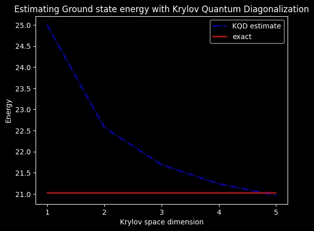
and get an estimate of the ground state energy $c_{min}$

gnd_en_circ_est_list = []
for d in range(1, krylov_dim + 1):
    # Solve generalized eigenvalue problem for different size of the Krylov space
    gnd_en_circ_est = solve_regularized_gen_eig(
        H_eff_circ[:d, :d], S_circ[:d, :d], threshold=9e-1
    )
    gnd_en_circ_est_list.append(gnd_en_circ_est)
    print("The estimated ground state energy is: ", gnd_en_circ_est)

Output:

The estimated ground state energy is:  25.0
The estimated ground state energy is:  22.572154819954875
The estimated ground state energy is:  21.691509219286587
The estimated ground state energy is:  21.23882298756386
The estimated ground state energy is:  20.965499325470294

For a single-particle sector, we can efficiently calculate the ground state of this sector of the Hamiltonian classically

gs_en = single_particle_gs(H_op, n_qubits)

Output:

n_sys_qubits 30
n_exc 1 , subspace dimension 31
single particle ground state energy:  21.021912418526906

plt.plot(
    range(1, krylov_dim + 1),
    gnd_en_circ_est_list,
    color="blue",
    linestyle="-.",
    label="KQD estimate",
)
plt.plot(
    range(1, krylov_dim + 1),
    [gs_en] * krylov_dim,
    color="red",
    linestyle="-",
    label="exact",
)
plt.xticks(range(1, krylov_dim + 1), range(1, krylov_dim + 1))
plt.legend()
plt.xlabel("Krylov space dimension")
plt.ylabel("Energy")
plt.title(
    "Estimating Ground state energy with Krylov Quantum Diagonalization"
)
plt.show()

Output:

Appendix: Krylov subspace from real time-evolutions

The unitary Krylov space is defined as

for some timestep $dt$ that we will determine later. Temporarily assume $r$ is even: then define $d=r/2$. Notice that when we project the Hamiltonian into the Krylov space above, it is indistinguishable from the Krylov space

i.e., where all the time-evolutions are shifted backward by $d$ timesteps. The reason it is indistinguishable is because the matrix elements

are invariant under overall shifts of the evolution time, since the time-evolutions commute with the Hamiltonian. For odd $r$, we can use the analysis for $r-1$.

We want to show that somewhere in this Krylov space, there is guaranteed to be a low-energy state. We do so by way of the following result, which is derived from Theorem 3.1 in [3]:

Claim 1: there exists a function $f$ such that for energies $E$ in the spectral range of the Hamiltonian (i.e., between the ground state energy and the maximum energy)...

1. $f(E_0)=1$
2. $|f(E)|\le2\left(1 + \delta\right)^{-d}$ for all values of $E$ that lie $\ge\delta$ away from $E_0$, i.e., it is exponentially suppressed
3. $f(E)$ is a linear combination of $e^{ijE\,dt}$ for $j=-d,-d+1,...,d-1,d$

We give a proof below, but that can be safely skipped unless one wants to understand the full, rigorous argument. For now we focus on the implications of the above claim. By property 3 above, we can see that the shifted Krylov space above contains the state $f(H)|\psi\rangle$. This is our low-energy state. To see why, write $|\psi\rangle$ in the energy eigenbasis:

where $|E_k\rangle$ is the kth energy eigenstate and $\gamma_k$ is its amplitude in the initial state $|\psi\rangle$. Expressed in terms of this, $f(H)|\psi\rangle$ is given by

using the fact that we can replace $H$ by $E_k$ when it acts on the eigenstate $|E_k\rangle$. The energy error of this state is therefore

To turn this into an upper bound that is easier to understand, we first separate the sum in the numerator into terms with $E_k-E_0\le\delta$ and terms with $E_k-E_0>\delta$:

We can upper bound the first term by $\delta$,

where the first step follows because $E_k-E_0\le\delta$ for every $E_k$ in the sum, and the second step follows because the sum in the numerator is a subset of the sum in the denominator. For the second term, first we lower bound the denominator by $|\gamma_0|^2$, since $f(E_0)^2=1$: adding everything back together, this gives

To simplify what is left, notice that for all these $E_k$, by the definition of $f$ we know that $f(E_k)^2 \le 4\left(1 + \delta\right)^{-2d}$. Additionally upper bounding $E_k-E_0<2\|H\|$ and upper bounding $\sum_{E_k>E_0+\delta}|\gamma_k|^2<1$ gives

This holds for any $\delta>0$, so if we set $\delta$ equal to our goal error, then the error bound above converges towards that exponentially with the Krylov dimension $2d=r$. Also note that if $\delta<E_1-E_0$ then the $\delta$ term actually goes away entirely in the above bound.

To complete the argument, we first note that the above is just the energy error of the particular state $f(H)|\psi\rangle$, rather than the energy error of the lowest energy state in the Krylov space. However, by the (Rayleigh-Ritz) variational principle, the energy error of the lowest energy state in the Krylov space is upper bounded by the energy error of any state in the Krylov space, so the above is also an upper bound on the energy error of the lowest energy state, i.e., the output of the Krylov quantum diagonalization algorithm.

A similar analysis as the above can be carried out that additionally accounts for noise and the thresholding procedure discussed in the notebook. See [2] and [4] for this analysis.

Appendix: proof of Claim 1

The following is mostly derived from [3], Theorem 3.1: let $0 < a < b$ and let $\Pi^*_d$ be the space of residual polynomials (polynomials whose value at 0 is 1) of degree at most $d$. The solution to

is

References

[1] N. Yoshioka, M. Amico, W. Kirby et al. "Diagonalization of large many-body Hamiltonians on a quantum processor". arXiv:2407.14431
[2] Ethan N. Epperly, Lin Lin, and Yuji Nakatsukasa. "A theory of quantum subspace diagonalization". SIAM Journal on Matrix Analysis and Applications 43, 1263–1290 (2022).
[3] Å. Björck. "Numerical methods in matrix computations". Texts in Applied Mathematics. Springer International Publishing. (2014).
[4] William Kirby. "Analysis of quantum Krylov algorithms with errors". Quantum 8, 1457 (2024).
Tutorial survey
Please take one minute to provide feedback on this tutorial. Your insights will help us improve our content offerings and user experience.