Exact simulation with Qiskit SDK primitives
The reference primitives in the Qiskit SDK perform local statevector simulations. These simulations do not support modeling device noise, but are useful for quickly prototyping algorithms before looking into more advanced simulation techniques (using Qiskit Aer) or running on real devices (Qiskit Runtime primitives).
The Estimator primitive can compute expectation values of circuits, and the Sampler primitive can sample from output distributions of circuits.
The following sections show how to use the reference primitives to run your workflow locally.
Use the reference Estimator
The reference implementation of EstimatorV2 in qiskit.primitives that runs on a local statevector
simulators is the StatevectorEstimator class. It can take circuits, observables, and parameters as inputs and returns the locally computed expectation values.
The following code prepares the inputs that will be used in the examples that follow. The expected input type for the
observables is qiskit.quantum_info.SparsePauliOp. Note that
the circuit in the example is parametrized, but you can also run the Estimator on non-parametrized circuits.
Any circuit passed to an Estimator must not include any measurements.
from qiskit import QuantumCircuit
from qiskit.circuit import Parameter

# circuit for which you want to obtain the expected value
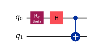
qc = QuantumCircuit(2)
qc.ry(Parameter('theta'), 0)
qc.h(0)
qc.cx(0,1)
qc.draw("mpl", style="iqp")
from qiskit.quantum_info import SparsePauliOp
import numpy as np

# observable(s) whose expected values you want to compute
from qiskit.quantum_info import SparsePauliOp
observable = SparsePauliOp(["II", "XX", "YY", "ZZ"], coeffs=[1, 1, -1, 1])

# value(s) for the circuit parameter(s)
parameter_values = [[0], [np.pi/6], [np.pi/2]]The Qiskit Runtime primitives workflow requires circuits and observables to be transformed to only use instructions supported by the QPU (referred to as instruction set architecture (ISA) circuits and observables). The reference primitives still accept abstract instructions, as they rely on local statevector simulations, but transpiling the circuit might still be beneficial in terms of circuit optimization.
# Generate a pass manager without providing a backend
from qiskit.transpiler.preset_passmanagers import generate_preset_pass_manager

pm = generate_preset_pass_manager(optimization_level=1)
isa_circuit = pm.run(qc)
isa_observable = observable.apply_layout(isa_circuit.layout)
Initialize Estimator
Instantiate a qiskit.primitives.StatevectorEstimator.
from qiskit.primitives import StatevectorEstimator
estimator = StatevectorEstimator()
Run and get results
This example only uses one circuit (of type QuantumCircuit) and one
observable.
Run the estimation by calling the StatevectorEstimator.run method, which returns an instance of a PrimitiveJob object. You can get the results from the job (as a qiskit.primitives.PrimitiveResult object)
with the qiskit.primitives.PrimitiveJob.result method.
job = estimator.run([(isa_circuit, isa_observable, parameter_values)])
result = job.result()
print(f" > Result class: {type(result)}")
> Result class: <class 'qiskit.primitives.containers.primitive_result.PrimitiveResult'>Get the expected value from the result
The primitives result outputs an array of PubResults, where each item of the array is a PubResult object that contains in its data the array of evaluations corresponding to every circuit-observable combination in the PUB.
To retrieve the expectation values and metadata for the first (and in this case, only) circuit evaluation, we must access the evaluation data for PUB 0:
print(f" > Expectation value: {result[0].data.evs}")
print(f" > Metadata: {result[0].metadata}")
> Expectation value: [4. 3.73205081 2. ]
> Metadata: {'precision': 0.0}Set Estimator run options
By default, the reference Estimator performs an exact statevector calculation based on the
quantum_info.Statevector class.
However, this can be modified to introduce the effect of the sampling overhead (also known as "shot noise").
Estimator accepts a precision argument that expresses the error bars that the
primitive implementation should target for expectation values estimates. This is the sampling overhead and is defined exclusively in the .run() method. This lets you fine-tune the option all the way to the PUB level.
This example assumes you have defined two circuits, each with its own array of observables.
# Estimate expectation values for two PUBs, both with 0.05 precision.
estimator.run([(isa_circuit1, isa_obs_array1), (isa_circuit2, isa_obs_array_2)], precision=0.05)
For a full example, see the Primitives examples page.
Use the reference Sampler
The reference implementations of SamplerV2 in qiskit.primitives is the StatevectorSampler class. It takes circuits and parameters as inputs and returns the results from sampling from the output probability distributions as a quasi-probability distribution of output states.
The following code prepares the inputs used in the examples that follow. Note that these examples run a single parametrized circuit, but you can also run the Sampler on non-parametrized circuits.
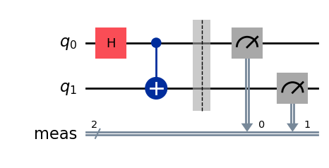
from qiskit import QuantumCircuit

qc = QuantumCircuit(2)
qc.h(0)
qc.cx(0,1)
qc.measure_all()
qc.draw("mpl", style="iqp")
Any quantum circuit passed to a Sampler must include measurements.
The Qiskit Runtime primitives workflow requires circuits to be transformed to only use instructions supported by the QPU (referred to as ISA circuits). The reference primitives still accept abstract instructions, as they rely on local statevector simulations, but transpiling the circuit might still be beneficial in terms of circuit optimization.
# Generate a pass manager without providing a backend
from qiskit.transpiler.preset_passmanagers import generate_preset_pass_manager

pm = generate_preset_pass_manager(optimization_level=1)
isa_circuit = pm.run(qc)
isa_observable = observable.apply_layout(isa_circuit.layout)
Initialize SamplerV2
Instantiate qiskit.primitives.StatevectorSampler:
from qiskit.primitives import StatevectorSampler

sampler = StatevectorSampler()
Run and get results
# execute 1 circuit with Sampler
job = sampler.run([isa_circuit])
pub_result = job.result()[0]
print(f" > Result class: {type(pub_result)}")
> Result class: <class 'qiskit.primitives.containers.pub_result.PubResult'>Primitives accept multiple PUBs as inputs, and each PUB gets its own result. Therefore, you can run different circuits with various parameter/observable combinations, and retrieve the PUB results:
from qiskit.transpiler.preset_passmanagers import generate_preset_pass_manager

# create two circuits
circuit1 = qc.copy()
circuit2 = qc.copy()

# transpile circuits
pm = generate_preset_pass_manager(optimization_level=1)
isa_circuit1 = pm.run(circuit1)
isa_circuit2 = pm.run(circuit2)
# execute 2 circuits using Sampler
job = sampler.run([(isa_circuit1), (isa_circuit2)])
pub_result_1 = job.result()[0]
pub_result_2 = job.result()[1]
print(f" > Result class: {type(pub_result)}")
> Result class: <class 'qiskit.primitives.containers.pub_result.PubResult'>Get the probability distribution or measurement outcome
Measurement outcome samples are returned as bitstrings or counts. The bitstrings show the measurement outcomes, preserving the shot order in which they were measured. The Sampler result objects organize data in terms of their input circuits' classical register names, for compatibility with dynamic circuits.
The name of the classical register defaults to "meas". This name will be used later to access the measurement bitstrings.
 # Define quantum circuit with 2 qubits
 circuit = QuantumCircuit(2)
 circuit.h(0)
 circuit.cx(0, 1)
 circuit.measure_all()
 circuit.draw()
┌───┐ ░ ┌─┐
q_0: ┤ H ├──■───░─┤M├───
└───┘┌─┴─┐ ░ └╥┘┌─┐
q_1: ─────┤ X ├─░──╫─┤M├
└───┘ ░ ║ └╥┘
meas: 2/══════════════╩══╩═
0 1# Transpile circuit
pm = generate_preset_pass_manager(optimization_level=1)
isa_circuit = pm.run(circuit)
# Run using sampler
result = sampler.run([circuit]).result()
# Access result data for PUB 0
data_pub = result[0].data
# Access bitstring for the classical register "meas"
bitstrings = data_pub.meas.get_bitstrings()
print(f"The number of bitstrings is: {len(bitstrings)}")
# Get counts for the classical register "meas"
counts = data_pub.meas.get_counts()
print(f"The counts are: {counts}")The number of bitstrings is: 1024
The counts are: {'11': 503, '00': 521}Change run options
By default, the reference Sampler performs an exact statevector calculation based on the
quantum_info.Statevector class.
However, this can be modified to introduce the effect of the sampling overhead (also known as "shot noise"). To help manage this overhead, the Sampler interface accepts a shots argument that can be defined at the PUB level.
This example assumes you have defined two circuits.
 # Sample two circuits at 128 shots each.
 sampler.run([isa_circuit1, isa_circuit2], shots=128)
 # Sample two circuits at different amounts of shots. The "None"s are necessary
 # as placeholders
 # for the lack of parameter values in this example.
 sampler.run([(isa_circuit1, None, 123), (isa_circuit2, None, 456)])
For a full example, see the Primitives examples page.
Next steps
- For higher-performance simulation that can handle larger circuits, or to incorporate noise models into your simulation, see Exact and noisy simulation with Qiskit Aer primitives.
- To learn how to use Quantum Composer for simulation, try the Explore gates and circuits with the Quantum Composer tutorial.
- Read the Qiskit Estimator API reference.
- Read the Qiskit Sampler API reference.
- Learn how to run on a QPU in the Run step of the Qiskit patterns workflow.
- Read Migrate to V2 primitives.