Grover's algorithm

For this Qiskit in Classrooms module, students must have a working Python environment with the following packages installed:

• qiskit v2.1.0 or newer
• qiskit-ibm-runtime v0.40.1 or newer
• qiskit-aer v0.17.0 or newer
• qiskit.visualization
• numpy
• pylatexenc

To set up and install the packages above, see the Install Qiskit guide. In order to run jobs on real quantum computers, students will need to set up an account with IBM Quantum® by following the steps in the Set up your IBM Cloud account guide.

This module was tested and used 12 seconds of QPU time. This is a good-faith estimate; your actual usage may vary.

# Uncomment and modify this line as needed to install dependencies
#!pip install 'qiskit>=2.1.0' 'qiskit-ibm-runtime>=0.40.1' 'qiskit-aer>=0.17.0' 'numpy' 'pylatexenc'

Introduction

Grover's algorithm is a foundational quantum algorithm that addresses the unstructured search problem: given a set of $N$ items and a way to check if any given item is the one you're looking for, how quickly can you find the desired item? In classical computing, if the data is unsorted and there is no structure to exploit, the best approach is to check each item one by one, leading to a query complexity of $O(N)$ — on average, you'll need to check about half the items before finding the target.

Grover's algorithm, introduced by Lov Grover in 1996, demonstrates how a quantum computer can solve this problem much more efficiently, requiring only $O(\sqrt{N})$ steps to find the marked item with high probability. This represents a quadratic speedup over classical methods, which is significant for large datasets.

The algorithm operates in the following context:

• Problem setup: You have a function $f(x)$ that returns 1 if $x$ is the item you want, and 0 otherwise. This function is often called an oracle or black box, since you can only learn about the data by querying $f(x)$.
• Usefulness of quantum: While classical algorithms for this problem require, on average, $N/2$ queries, Grover's algorithm can find the solution in roughly $\pi\sqrt{N}/4$ queries, which is much faster for large $N$.
• How it works (at a high level):
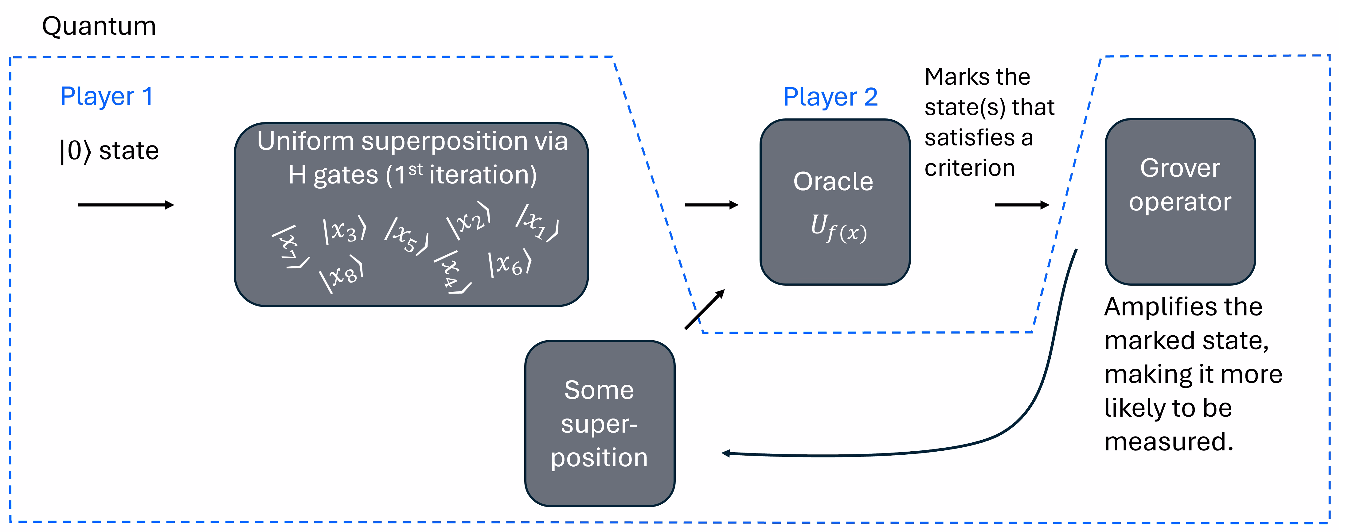
  • The quantum computer first creates a superposition of all possible states, representing all possible items at once.
  • It then repeatedly applies a sequence of quantum operations (the Grover iteration) that amplifies the probability of the correct answer and diminishes the others.
  • After enough iterations, measuring the quantum state yields the correct answer with high probability.

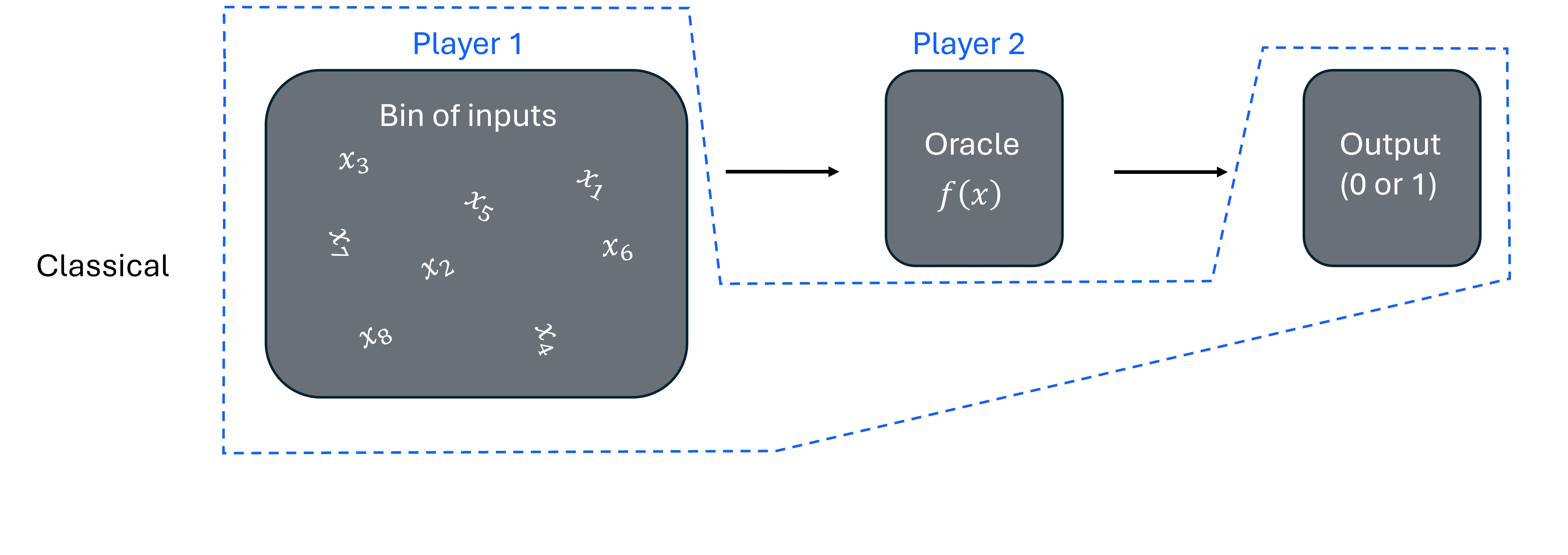
Here is a very basic diagram of Grover's algorithm that skips over a lot of nuance. For a more detailed diagram, see this paper.

A few things to note about Grover's algorithm:

• It is optimal for unstructured search: no quantum algorithm can solve the problem with fewer than $O(\sqrt{N})$ queries.
• It provides only a quadratic, not exponential, speedup — unlike some other quantum algorithms (for example, Shor's algorithm for factoring).
• It has practical implications, such as potentially speeding up brute-force attacks on cryptographic systems, though the speedup is not enough to break most modern encryption by itself.

For undergraduate students familiar with basic computing concepts and query models, Grover's algorithm offers a clear illustration of how quantum computing can outperform classical approaches for certain problems, even when the improvement is "only" quadratic. It also serves as a gateway to understanding more advanced quantum algorithms and the broader potential of quantum computing.

Amplitude amplification is a general purpose quantum algorithm, or subroutine, that can be used to obtain a quadratic speedup over a handful of classical algorithms. Grover’s algorithm was the first to demonstrate this speedup on unstructured search problems. Formulating a Grover's search problem requires an oracle function that marks one or more computational basis states as the states we are interested in finding, and an amplification circuit that increases the amplitude of marked states, consequently suppressing the remaining states.

Here, we demonstrate how to construct Grover oracles and use the GroverOperator from the Qiskit circuit library to easily set up a Grover's search instance. The runtime Sampler primitive allows seamless execution of Grover circuits.

Theory

Suppose there exists a function $f$ that maps binary strings to a single binary variable, meaning

One example defined on $\Sigma^6$ is

Another example defined on $\Sigma^{2n}$ is

You are tasked with finding quantum states corresponding to those arguments $x$ of $f(x)$ that are mapped to 1. In other words, find all $\{x_1\}\in \Sigma^n$ such that $f(x_1)=1$ (or if there is no solution, report that). We would refer to non-solutions as $x_0$. Of course, we will do this on a quantum computer, using quantum states, so it is useful to express these binary strings as states:

Using the quantum state (Dirac) notation, we are looking for one or more special states $\{|x_1\rangle\}$ in a set of $N=2^n$ possible states, where $n$ is the number of qubits, and with non-solutions denoted $\{|x_0\rangle\}.$

We can think of the function $f$ as being provided by an oracle: a black-box that we can query to determine its effect on a state $|x\rangle.$ In practice, we will often know the function, but it may be very complicated to implement, meaning that reducing the number of queries or applications of $f$ could be important. Alternatively, we can imagine a paradigm in which one person is querying an oracle controlled by another person, such that we don't know the oracle function, we only know its action on particular states from querying.

This is an "unstructured search problem, in that there is nothing special about $f$ that aids us in our search. The outputs are not sorted nor are solutions known to cluster, and so on. Consider use old, paper phone books as an analogy. This unstructured search would be like scanning through it looking for a certain number, and not like looking through an alphabetized list of names.

In the case where a single solution is sought, classically, this requires a number of queries that is linear in $N$. Clearly you might find a solution on the first try, or you might find no solutions in the first $N-1$ guesses, such that you need to query the $N^{th}$ input to see if there is any solution at all. Since the functions have no exploitable structure, you will require $N/2$ guesses on average. Grover's algorithm requires a number of queries or computations of $f$ that scales like $\sqrt{N}.$

Sketch of circuits in Grover's algorithm

A full mathematical walkthrough of Grover's algorithm can be found, for example, in Fundamentals of quantum algorithms, a course by John Watrous on IBM Quantum Learning. A condensed treatment is provided in an appendix at the end of this module. But for now, we will only review the overall structure of the quantum circuit that implements Grover's algorithm.

Grover's algorithm can be broken down into the following stages:

• Preparation of an initial superposition (applying Hadamard gates to all qubits)
• "Marking" the target state(s) with a phase flip
• A "diffusion" stage in which Hadamard gates and a phase flip are applied to all qubits.
• Possible repetitions of the marking and diffusion stages to maximize the probability of measuring the target state
• Measurement

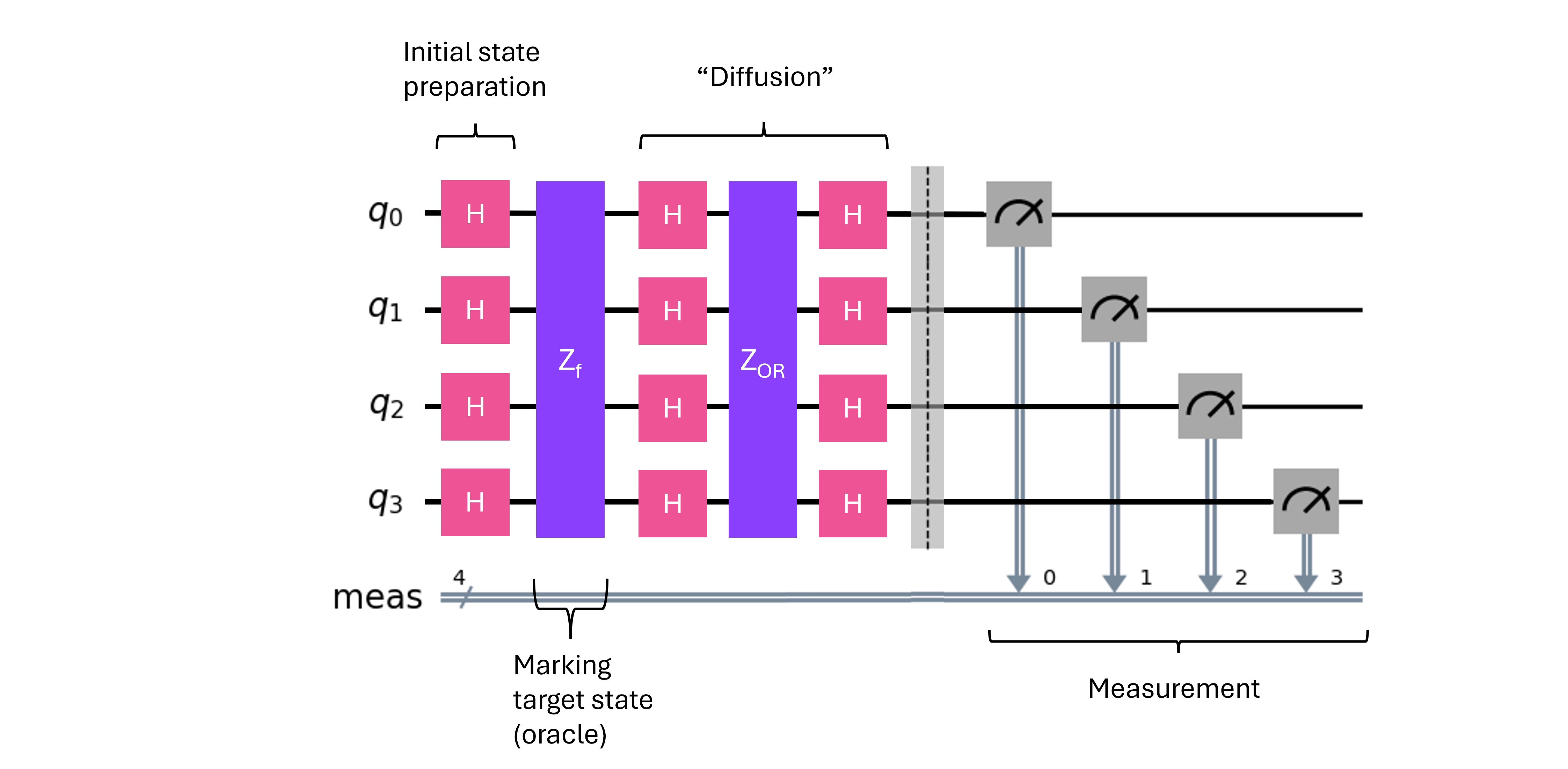
Often, the marking gate $Z_f$ and the diffusion layers consisting of $H,$ $Z_{\text{OR}},$ and $H$ are collectively referred to as the "Grover operator". In this diagram, only a single repetition of the Grover operator is shown.

Hadamard gates $H$ are well-known and used widely throughout quantum computing. The Hadamard gate creates superposition states. Specifically it is defined by

Its operation on any other state is defined through linearity. In particularly, a layer of Hadamard gates allows us to go from the initial state with all qubits in $|0\rangle$ (denoted $|0\rangle^{\otimes n}$) to a state where each qubit has some probability of being measured in either $|0\rangle$ or $|1\rangle;$ this lets us probe the space of all possible states differently from in classical computing.

An important corollary property of the Hadamard gate is that acting a second time can undo such superposition states:

This will be important in just a moment.

Check your understanding

Starting from the definition of the Hadamard gate, demonstrate that a second application of the Hadamard gate undoes such superpositions as claimed above.

• Answer

  When we apply X to the $|+\rangle$ state, we get the value and +1 and to the state $|-\rangle$ we get -1, so if we had a 50-50 distribution, we would get an expectation value of 0.

The $Z_\text{OR}$ gate is less common, and is defined according to

Finally, the $Z_f$ gate is defined by

Note the effect of this is that $Z_f$ flips the sign on a target state for which $f(x) = 1$ and leaves other states unaffected.

At a very high, abstract level you can think about the steps in the circuit in the following ways:

• First Hadamard layer: puts the qubits into a superposition of all possible states.
• $Z_f$: mark the target state(s) by adding a "-" sign in front. This doesn't immediately change measurement probabilities, but it changes how the target state will behave in subsequent steps.
• Another Hadamard layer: The "-" sign introduced in the previous step will change the relative sign between some terms. Since Hadamard gates turn one mixture of computational states $(|0\rangle+|1\rangle)/\sqrt{2}$ into one computational state, $|0\rangle,$ and they turn $(|0\rangle-|1\rangle)/\sqrt{2}$ into $|1\rangle$ this relative sign difference can now begin to play a role in what states are measured.
• One final layer of Hadamard gates is applied, and then measurements are made. We will see in more detail how this works in the next section.

Example

To better understand how Grover's algorithm works, let us work through a small, two-qubit example. This may be considered optional for those not focused on quantum mechanics and Dirac notation. But for those who hope to work substantially with quantum computers, this is highly recommended.

Here is the circuit diagram with the quantum states labeled at various positions throughout. Note that with only two qubits, there are only four possible states that could be measured under any circumstances: $|00\rangle$, $|01\rangle$, $|10\rangle$, and $|11\rangle$.

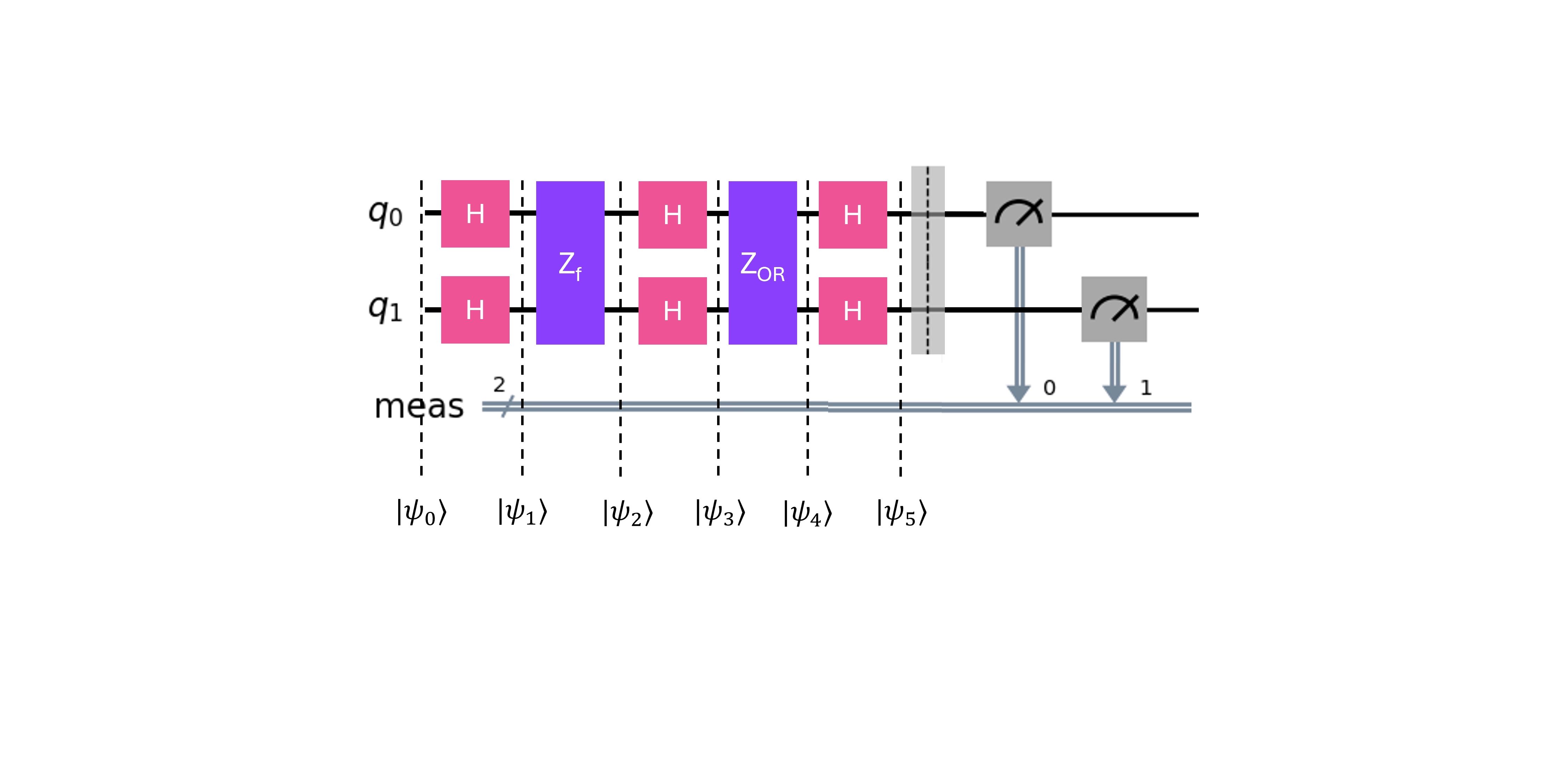
Let us suppose that the oracle ($Z_f$, unknown to us) marks the state $|01\rangle$. We will work through the actions of each set of quantum gates, including the oracle, and see what distribution of possible states come out at the time of measurement. At the very beginning, we have

Using the definition of Hadamard gates, we have

Now the oracle marks the target state:

Note that in this state, all four possible outcomes have the same probability of being measured. They all have a weight of magnitude $1/2,$ meaning they each have a $|1/2|^2=1/4$ chance of being measured. So while the state $|01\rangle$ is marked through the "-" phase, this has not yet resulted in any increased probability of measuring that state. We continue by applying the next layer of Hadamard gates.

Combining like terms, we find

Now $Z_{\text{OR}}$ flips the sign on all states but $|00\rangle$:

And finally, we apply the last layer of Hadamard gates:

It is worth working through the combining of these terms to convince yourself that the result is indeed:

That is, the probability of measuring $|01\rangle$ is 100% (in the absence of noise and errors) and the probability for measuring any other state is zero.

This two-qubit example was an especially clean case; Grover's algorithm will not always work out to yield a 100% chance of measuring the target state. Rather, it will amplify the probability of measuring the target state. Also, the Grover operator may need to be repeated more than once.

In the next section, we will put this algorithm into practice using real IBM® quantum computers.

The geometric picture

The two-qubit example above showed how the algebra works out for a small case, but there is a much more intuitive way to understand Grover's algorithm: as a sequence of geometric reflections in a two-dimensional plane. Below we describe this picture. You can also see John Watrous's course Fundamentals of Quantum Algorithms for more details.

Setting up the plane. We can decompose the initial superposition state $|\psi\rangle$ into two components. The correct state — the one we're searching for — we call $|A_1\rangle$. Every other state, lumped together, we call $|A_0\rangle$. By definition, $|A_1\rangle$ and $|A_0\rangle$ are orthogonal to one another, so we can plot them as perpendicular axes in an abstract, two-dimensional space. Since $|\psi\rangle$ is a linear combination of these two components, it sits at some small angle $\theta$ to the $|A_0\rangle$ axis — close to $|A_0\rangle$, because at the start, only a tiny fraction of the state is in the correct component $|A_1\rangle$.

Reflections. The key mathematical fact we need is that an operator of the form

reflects any state about the axis defined by $|v\rangle.$ To see why, consider two cases: a state along $|v\rangle$ is left unchanged, and a state perpendicular to $|v\rangle$ gets its sign flipped. Any other state can be decomposed into these two components, and the operator acts on each accordingly — which is exactly a reflection about $|v\rangle$.

It turns out that both the oracle and the diffusion steps in Grover's algorithm can be expressed as reflections in this geometric picture.

The oracle as a reflection. The oracle flips the sign of the $|A_1\rangle$ state and leaves everything else alone. That is the same as a reflection about the $|A_0\rangle$ axis.

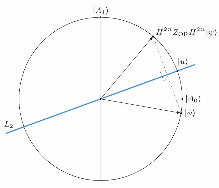
Diffusion as a reflection. It is a little trickier to see how the diffusion operator is also a reflection. The diffusion operator is

$Z_{\text{OR}}$ by itself is a reflection about the all-zero state, since it flips the sign of every state that is not $|0\rangle^{\otimes n}$. This can be written as $2|0\rangle\langle 0| - I$. The surrounding Hadamard layers effectively perform a change of basis, transforming the axis of reflection. Recall that $H^{\otimes n}$ maps $|0\rangle^{\otimes n}$ to the uniform superposition $|u\rangle = \frac{1}{\sqrt{N}}\sum_{x}|x\rangle$. Since the Hadamard is its own inverse, the full expression becomes

which is a reflection about $|u\rangle$. Since $|u\rangle$ is very close to $|\psi\rangle$ (both are nearly along $|A_0\rangle$), this second reflection sends the state to an angle $2\theta$ from where it started.

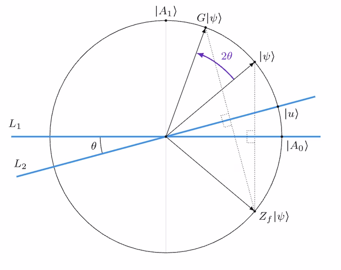
Rotation by $2\theta$. The combined effect of these two reflections is a rotation by $2\theta$ toward $|A_1\rangle$. Each successive iteration of the Grover operator rotates the state by another $2\theta.$

Optimal number of iterations. Our goal is to rotate the state as close to $|A_1\rangle$ as possible, which means rotating by a total of approximately $\pi/2$ radians (a quarter turn). If each iteration contributes $2\theta$, the optimal number of iterations $t$ satisfies

For a single solution among $N$ states, the initial angle is $\theta \approx \sin^{-1}(1/\sqrt{N}) \approx 1/\sqrt{N}$ (for large $N$). Substituting,

This is where the famous $\sqrt{N}$ speedup comes from: we only need $O(\sqrt{N})$ iterations to reach the target, rather than the $O(N)$ checks a classical search would require.

More generally, if there are $|A_1|$ solution states among $N$ total states, the optimal number of iterations is

Note that if you apply too many iterations, you rotate past $|A_1\rangle$ and the probability of finding your target state will start to decrease again. Finding the right number of iterations is important, though on noisy quantum hardware the experimentally optimal number may differ from this ideal formula.

Why is Grover's algorithm useful?

At this point you may be wondering: we just built an oracle that marks a target state — but to build it, we had to know the target state. So what are we actually searching for?

This is a fair question, and there are several good answers.

• The query model is a theoretical tool. The query model of computation was never designed to be directly practical. Its purpose is to give us a clean way to analyze algorithmic complexity by separating a problem into two parts: the oracle, and everything else. How hard is the search, given that verification is free? How does the number of queries scale with the size of the input? These are useful questions even if no real system works exactly this way.

• You can also think of it as a two-party activity: one person knows the target state and builds the oracle; the other person's job is to find the answer using the oracle as a black box, with no peeking inside. In Activity 2 below, you will do exactly this with a partner.

• Amplitude amplification is a broadly useful subroutine. Even if this first demonstration seems circular, the underlying mechanism — called amplitude amplification — shows up again and again in quantum computing. What we are really building here is an intuition for a tool that appears as a subroutine in many more complex quantum algorithms.

• There are problems where you can build an oracle without knowing the answer. The key insight is that there exists a whole class of problems for which it is very hard to find a solution, but very easy to check that a given solution is correct. Factoring is one example: given a product of two large primes, it is extremely difficult to determine what those primes are, but once you have them, you can easily multiply them together to verify. (We have a better algorithm than Grover's for factoring specifically — see Shor's algorithm — but this is far from the only problem with this feature.) Sudoku, constraint satisfaction, and even the classic game of Minesweeper are all problems that are difficult to solve but easy to check.

Why is that relevant? It means we can know all of the conditions and requirements that a solution must satisfy, and we can encode those requirements into a quantum circuit that serves as the oracle — even though we do not know the solution itself. Grover's algorithm will find it for us.

With these ideas in mind, let us work through several examples. We will begin with an example in which the solution state is clearly specified so we can follow the logic of the algorithm. We will then move on to a two-party activity, and finally to an example in which the oracle is built from problem constraints rather than from knowledge of the answer.

General imports and approach

We start by importing several necessary packages.

# Built-in modules
import math

# Imports from Qiskit
from qiskit import QuantumCircuit, QuantumRegister, ClassicalRegister
from qiskit.circuit.library import grover_operator, MCMTGate, ZGate
from qiskit.visualization import plot_distribution
from qiskit.transpiler.preset_passmanagers import generate_preset_pass_manager

Throughout this and other tutorials, we will use a framework for quantum computing known as "Qiskit patterns", which breaks workflows into the following steps:

• Step 1: Map classical inputs to a quantum problem
• Step 2: Optimize problem for quantum execution
• Step 3: Execute using Qiskit Runtime Primitives
• Step 4: Post-processing and classical analysis

We will generally follow these steps, though we may not always explicitly label them.

Activity 1: Find a single given target state

Step 1: Map classical inputs to a quantum problem

We need the phase query gate to put an overall phase (-1) on solution states, and leave the non-solution states unaffected. Another way of saying this is that Grover's algorithm requires an oracle that specifies one or more marked computational basis states, where "marked" means a state with a phase of -1. This is done using a controlled-Z gate, or its multi-controlled generalization over $N$ qubits. To see how this works, consider a specific example of a bitstring {110}. We would like a circuit that acts on a state $|\psi\rangle = |q_2,q_1,q_0\rangle$ and applies a phase if $|\psi\rangle = |011\rangle$ (where we have flipped the order of the binary string, because of the notation in Qiskit, which puts the least significant (often 0) qubit on the right).

Thus, we want a circuit $Z_f$ that accomplishes

We can use the multiple control multiple target gate (MCMTGate) to apply a Z gate controlled by all qubits (flip the phase if all qubits are in the $|1\rangle$ state). Of course, some of the qubits in our desired state may be $|0\rangle$. Therefore, for those qubits we must first apply an X gate, then do the multiply-controlled Z gate, then apply another X gate to undo our change. The MCMTGate looks like this:

mcmt_ex = QuantumCircuit(3)
mcmt_ex.compose(MCMTGate(ZGate(), 3 - 1, 1), inplace=True)
mcmt_ex.draw(output="mpl", style="iqp")

Output:

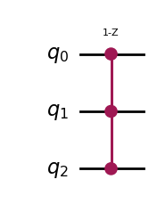
Note that many qubits may be involved in the control process (here three qubits are), but no single qubit is denoted as a target. This is because the entire state gets an overall "-" sign (phase flip); the gate affects all the qubits equivalently. This is different from many other multiple qubit gates, like the CX gate, which has a single control qubit and a single target qubit.

In the following code, we define a phase query gate (or oracle) that does what we just described above: marks one or more input basis states defined through their bitstring representation. The MCMT gate is used to implement the multi-controlled Z-gate.

def grover_oracle(marked_states):
    """Build a Grover oracle for multiple marked states

    Here we assume all input marked states have the same number of bits

    Parameters:
        marked_states (str or list): Marked states of oracle

    Returns:
        QuantumCircuit: Quantum circuit representing Grover oracle
    """
    if not isinstance(marked_states, list):
        marked_states = [marked_states]
    # Compute the number of qubits in circuit
    num_qubits = len(marked_states[0])

    qc = QuantumCircuit(num_qubits)
    # Mark each target state in the input list
    for target in marked_states:
        # Flip target bitstring to match Qiskit bit-ordering
        rev_target = target[::-1]
        # Find the indices of all the '0' elements in bitstring
        zero_inds = [
            ind for ind in range(num_qubits) if rev_target.startswith("0", ind)
        ]
        # Add a multi-controlled Z-gate with pre- and post-applied X-gates (open-controls)
        # where the target bitstring has a '0' entry
        qc.x(zero_inds)
        qc.compose(MCMTGate(ZGate(), num_qubits - 1, 1), inplace=True)
        qc.x(zero_inds)
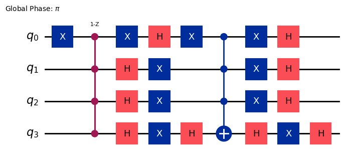
    return qc

Now we choose a specific "marked" state to be our target, and apply the function we just defined. Let's see what kind of circuit it created.

marked_states = ["1110"]
oracle = grover_oracle(marked_states)
oracle.draw(output="mpl", style="iqp")

Output:

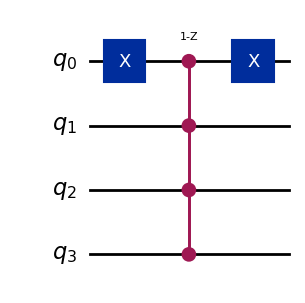
If qubits 1-3 are in the $|1\rangle$ state, and qubit 0 is initially in the $|0\rangle$ state, the first X gate will flip qubit 0 to $|1\rangle$ and all qubits will be in $|1\rangle.$ This means the MCMT gate will apply an overall sign change or phase flip, as desired. For any other case, either qubits 1-3 are in the $|0\rangle$ state, or qubit 0 is flipped to the $|0\rangle$ state, and the phase flip will not be applied. We see that this circuit does indeed mark our desired state $|0111\rangle,$ or the bitstring {1110}.

The full Grover operator consists of the phase query gate (oracle), Hadamard layers, and the $Z_\text{OR}$ operator. We can use the built-in grover_operator to construct this from the oracle we defined above.

grover_op = grover_operator(oracle)
grover_op.decompose(reps=0).draw(output="mpl", style="iqp")

Output:

As we discussed in the geometric picture above, we might need to apply the Grover operator multiple times. The optimal number of iterations $t$ to maximize the amplitude of the target state in the absence of noise is

where $|A_1|$ is the number of solution states and $N=2^n$ is the total number of states. On modern noisy quantum computers, the experimentally optimal number of iterations might be different — but here we calculate and use this theoretical, optimal number using $|A_1|=1$.

optimal_num_iterations = math.floor(
    math.pi / (4 * math.asin(math.sqrt(len(marked_states) / 2**grover_op.num_qubits)))
)
print(optimal_num_iterations)

Output:

3

Let us now construct a circuit that includes the initial Hadamard gates to create a superposition of all possible states, and apply the Grover operator the optimal number of times.

qc = QuantumCircuit(grover_op.num_qubits)
# Create even superposition of all basis states
qc.h(range(grover_op.num_qubits))
# Apply Grover operator the optimal number of times
qc.compose(grover_op.power(optimal_num_iterations), inplace=True)
# Measure all qubits
qc.measure_all()
qc.draw(output="mpl", style="iqp")

Output:

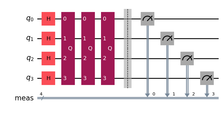
We have constructed our Grover circuit!

Step 2: Optimize problem for quantum hardware execution

We have defined our abstract quantum circuit, but we need to rewrite it in terms of gates that are native to the quantum computer we actually want to use. We also need to specify which qubits on the quantum computer should be used. For these reasons and others, we now must transpile our circuit. First, let us specify the quantum computer we wish to use.

There is code below for saving your credentials upon first use. Be sure to delete this information from the notebook after saving it to your environment, so that your credentials are not accidentally shared when you share the notebook. See Set up your IBM Cloud account and Initialize the service in an untrusted environment for more guidance.

# To run on hardware, select the backend with the fewest number of jobs in the queue
from qiskit_ibm_runtime import QiskitRuntimeService

# Syntax for first saving your token.  Delete these lines after saving your credentials.
# QiskitRuntimeService.save_account(channel='ibm_quantum_platform', instance = '<YOUR_IBM_INSTANCE_CRN>', token='<YOUR_API_KEY>', overwrite=True, set_as_default=True)
# service = QiskitRuntimeService(channel='ibm_quantum_platform')

# Load saved credentials
service = QiskitRuntimeService()

backend = service.least_busy(operational=True, simulator=False)
backend.name

Output:

qiskit_runtime_service._resolve_cloud_instances:WARNING:2025-08-08 14:14:19,931: Default instance not set. Searching all available instances.

'ibm_brisbane'

Now we use a preset pass manager to optimize our quantum circuit for the backend we selected.

target = backend.target
pm = generate_preset_pass_manager(target=target, optimization_level=3)

circuit_isa = pm.run(qc)
# The transpiled circuit will be very large. Only draw it if you are really curious.
# circuit_isa.draw(output="mpl", idle_wires=False, style="iqp")

It is worth noting at this time that the depth of the transpiled quantum circuit is substantial.

print("The total depth is ", circuit_isa.depth())
print(
    "The depth of two-qubit gates is ",
    circuit_isa.depth(lambda instruction: instruction.operation.num_qubits == 2),
)

Output:

The total depth is  439
The depth of two-qubit gates is  113

These are actually quite large numbers, even for this simple case. Since all quantum gates (and especially two-qubit gates) experience errors and are subject to noise, a series of over 100 two-qubit gates would result in nothing but noise if the qubits were not extremely high-performing. Let's see how these perform.

Step 3: Execute using Qiskit primitives

We want to make many measurements and see which state is the most likely. Such an amplitude amplification is a sampling problem that is suitable for execution with the Sampler Qiskit Runtime primitive.

Note that the run() method of Qiskit Runtime SamplerV2 takes an iterable of primitive unified blocks (PUBs). For Sampler, each PUB is an iterable in the format (circuit, parameter_values). However, at a minimum, it takes a list of quantum circuit(s).

# To run on a real quantum computer (this was tested on a Heron r2 processor and used 4 sec. of QPU time)

from qiskit_ibm_runtime import SamplerV2 as Sampler

sampler = Sampler(mode=backend)
sampler.options.default_shots = 10_000
result = sampler.run([circuit_isa]).result()
dist = result[0].data.meas.get_counts()

To get the most out of this experience, we highly recommend you run your experiments on the real quantum computers available from IBM Quantum. However, if you have exhausted your QPU time, you can uncomment the lines below to complete this activity using a simulator.

# To run on local simulator:
# from qiskit.primitives import StatevectorSampler as Sampler
# sampler = Sampler()
# result = sampler.run([qc]).result()
# dist = result[0].data.meas.get_counts()

Step 4: Post-process and return result in desired classical format

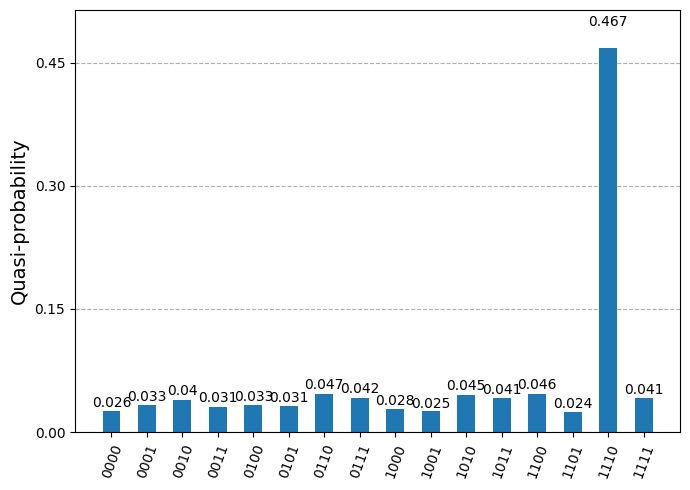
Now we can plot the results of our sampling in a histogram.

plot_distribution(dist)

Output:

We see that Grover's algorithm returned the desired state with the highest probability by far, at least an order of magnitude higher than other options. In the next activity, we will use the algorithm in a way that is more consistent with the two-party workflow of a query algorithm.

Check your understanding

We just searched for a single solution in a set of $2^4=16$ possible states. We determined the optimal number of repetitions of the Grover operator to be $t=3$. Would this optimal number have increased or decreased if we had searched for (a) any of several solutions, or (b) a single solution in a space of more possible states?

• Answer

  Recall that as long as the number of solutions is small compared to the entire space of solutions, we can expand the sine function around small angles and use

  $$(2t+1)\theta = (2t+1) \sin^{-1}{\sqrt{\frac{|\mathcal{A}_1|}{N}}}\approx (2t+1) \sqrt{\frac{|\mathcal{A}_1|}{N}} \approx \pi/2\\ t \approx \frac{\pi}{4}\sqrt{\frac{N}{|\mathcal{A}_1|}}-\frac{1}{2}$$

  (a) We see from the above expression that increasing the number of solution states would decrease the number of iterations. Provided that the fraction $\frac{|\mathcal{A}_1|}{N}$ is still small, we can describe how $t$ would decrease: $t~\frac{1}{\sqrt{|\mathcal{A}_1|}}.$

  (b) As the space of possible solutions ($N$) increases, the number of required iterations increases, but only like $t~\sqrt{N}$.

Suppose we could increase the size of the target bitstring to be arbitrarily long and still have the outcome that the target state has a probability amplitude that is at least an order of magnitude larger than any other state. Does this mean we could use Grover's algorithm to reliably find the target state?

• Answer

  No. Suppose we repeated the first activity with 20 qubits, and we run the quantum circuit a number of times num_shots = 10,000. A uniform probability distribution would mean that every state has a probability of $10,000/2^{20}=0.00954$ of being measured even a single time. If the probability of measuring the target state were 10 times that of non-solutions (and the probability of each non-solution were correspondingly slightly decreased), there would only be about a 10% chance of measuring the target state even once. It would be highly unlikely to measure the target state multiple times, which would make it indistinguishable from the many randomly-obtained non-solution states. The good news is that we can obtain even higher-fidelity results by using error suppression and mitigation.

Activity 2: An accurate query algorithm workflow

We will start this activity exactly as the first one, except that now you will pair up with another Qiskit enthusiast. You will pick a secret bitstring, and your partner will pick a (generally) different bitstring. You will each generate a quantum circuit that functions as an oracle, and you will exchange them. You will then use Grover's algorithm with that oracle to determine your partner's secret bitstring.

Step 1: Map classical inputs to a quantum problem

Using the grover_oracle function defined above, construct an oracle circuit for one or more marked states. Make sure you tell your partner how many states you have marked, so they can apply the Grover operator the optimal number of times. Don't make your bitstring too long. 3-5 bits should work without much difficulty. Longer bitstrings would result in deep circuits that require more advanced techniques like error mitigation.

# Modify the marked states to mark those you wish to target.
marked_states = ["1000"]
oracle = grover_oracle(marked_states)

Now you have created a quantum circuit that flips the phase of your target state. You can save this circuit as my_circuit.qpy using the syntax below.

from qiskit import qpy

# Save to a QPY file at a location where you can easily find it.
# You might want to specify a global address.
with open("C:\\Users\\...put your own address here...\\my_circuit.qpy", "wb") as f:
    qpy.dump(oracle, f)

Now send this file to your partner (via email, messaging service, a shared repo, and so forth). Have your partner send you their circuit as well. Make sure you save the file somewhere you can easily find it. Once you have your partner's circuit, you could visualize it - but that breaks the query model. That is, we're modeling a situation in which you can query the oracle (use the oracle circuit) but not examine it to determine what state it targets.

from qiskit import qpy

# Load the circuit from your partner's qpy file from the folder where you saved it.
with open("C:\\Users\\...file location here...\\my_circuit.qpy", "rb") as f:
    circuits = qpy.load(f)

# qpy.load always returns a list of circuits
oracle_partner = circuits[0]

# You could visualize the circuit, but this would break the model of a query algorithm.
# oracle_partner.draw("mpl")

Ask your partner how many target states they encoded and enter it below.

# Update according to your partner's number of target states.
num_marked_states = 1

This is used in the next expression to determine the optimal number of Grover iterations.

grover_op = grover_operator(oracle_partner)
optimal_num_iterations = math.floor(
    math.pi / (4 * math.asin(math.sqrt(num_marked_states / 2**grover_op.num_qubits)))
)
qc = QuantumCircuit(grover_op.num_qubits)
qc.h(range(grover_op.num_qubits))
qc.compose(grover_op.power(optimal_num_iterations), inplace=True)
qc.measure_all()

Step 2: Optimize problem for quantum hardware execution

This proceeds exactly as before.

# To run on hardware, select the backend with the fewest number of jobs in the queue
service = QiskitRuntimeService()
backend = service.least_busy(operational=True, simulator=False)
backend.name

target = backend.target
pm = generate_preset_pass_manager(target=target, optimization_level=3)
circuit_partner_isa = pm.run(qc)

Step 3: Execute using Qiskit primitives

This is also identical to the process in the first activity.

# To run on a real quantum computer (this was tested on a Heron r2 processor and used 4 seconds of QPU time)

from qiskit_ibm_runtime import SamplerV2 as Sampler

sampler = Sampler(mode=backend)
sampler.options.default_shots = 10_000
result = sampler.run([circuit_partner_isa]).result()
dist = result[0].data.meas.get_counts()

Step 4: Post-process and return result in desired classical format

Now display a histogram of your sampling results. One or more states should have much higher measurement probability than the others. Report these to your partner and check if you correctly determined the target states. By default, the histogram displayed is of the same circuit from the first activity. You should obtain different results from your partner's circuit.

plot_distribution(dist)

Output:

Check your understanding

You should have correctly obtained your partner's target state(s). If you did not, work with your partner to identify what went wrong. Click below for a few ideas.

• Hints
  • Visualize/draw your partner's circuit and make sure it loaded correctly.
  • Compare the circuits used and compare the expected outcome to that which you obtained.
  • Check the depth of the circuits used to make sure the bitstring wasn't too long or the number of Grover iterations prohibitively high.

If you haven't already, draw the oracle circuit your partner sent you. See if you can talk through the effect of each gate and argue what the target state must have been. This will be much easier for the case of a single marked state than for multiple.

• Hints
  • Recall that the job of the oracle is to flip the sign on the target state.
  • Recall that the MCMTGate flips the sign on a state if and only if all qubits involved in the control are in the $|1\rangle$ state.
  • If your target state will already have a $|1\rangle$ on a particular qubit, then you need not do anything to that qubit. If your target has a $|0\rangle$ on a particular qubit and you want the MCMTGate to flip the sign, you need to apply an X gate to that qubit in your oracle (and then undo the X gate after the MCMTGate).

Repeat the experiment with one fewer iteration of the Grover operator. Do you still obtain the correct answer? Why or why not?

• Guidance

  You probably will, though it might depend on the number of solutions encoded. This highlights a subtlety: the "optimal" number of Grover iterations is the number that makes the probability of measuring the marked state as high as possible. But fewer iterations than that might still make the marked state substantially more likely than other states. Therefore, you might be able to get away with fewer iterations than the optimal number. This reduces circuit depth, and thus reduces error rates.

Why might someone want to use fewer Grover iterations than the "optimal number" identified here?

• Answer

  The "optimal" number of Grover iterations is the number that makes the probability of measuring the marked state as high as possible in the absence of noise. But fewer iterations than that might still make the marked state substantially more likely than other states. So you might be able to get away with fewer iterations than the optimal number. This reduces circuit depth, and thus reduces error rates.

Activity 3: Solve a Minesweeper grid with Grover's algorithm

In the previous section, we noted that Grover's algorithm becomes genuinely useful when we can build an oracle from the constraints of a problem, rather than from knowledge of the answer. Minesweeper is a perfect example: the numbered cells tell us how many mines are adjacent, and those constraints fully determine where the mines must be — but finding the configuration requires search.

Minesweeper has been proven to be NP-complete: it is hard to solve but easy to check. That makes it a natural candidate for Grover's algorithm. Of course, we cannot yet solve a full 9$\times$9 grid on a noisy quantum computer — the circuits would be far too deep. Instead, we will use a tiny grid as a toy demonstration of how one would approach a larger board on a future fault-tolerant machine.

A few important caveats. Grover's algorithm provides only a quadratic speedup over unstructured classical search. Minesweeper almost certainly has exploitable structure that a clever classical algorithm could use. And for an exponentially growing search space, even the $\sqrt{N}$ improvement only goes so far. But let us set those concerns aside and use this toy problem to illustrate how problem constraints get encoded into a quantum oracle.

The grid

Here is our baby minesweeper grid:

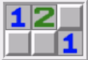
Each blank cell can be represented by a binary variable indicating whether it contains a mine. We label these $x_0$, $x_1$, and $x_2$, where $x_i = 1$ means there is a mine on that cell and $x_i = 0$ means there is not:

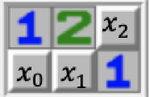
We could solve this in our heads in about half a second, but we are using this toy problem to illustrate how a much harder board could be approached with a quantum computer.

Encode the constraints

Each numbered cell places a condition on the adjacent blank cells. We need to express these conditions as Boolean expressions that can be encoded into a quantum circuit.

The "1" cell adjacent to $x_0$ and $x_1$ says that exactly one of them contains a mine. This is precisely the exclusive-OR (XOR) operation, $\oplus$, which returns true when exactly one of its inputs is true:

Similarly, the other "1" cell (adjacent to $x_1$ and $x_2$) gives us:

The "2" cell says that two of the three blank cells must contain mines. Since XOR is a parity operation, $x_0 \oplus x_1 \oplus x_2$ returns true when an odd number of the variables are true. We want an even number (specifically two) to be true, so we negate with $\lnot$:

On its own, this expression would be satisfied by either zero or two qubits in the $|1\rangle$ state, since it is a statement about parity. But combined with the other two clauses, which each require at least one mine, the only satisfying assignment has exactly two mines.

All three conditions must be simultaneously satisfied, so we join them with and symbols $\land$:

Step 1: Map classical inputs to a quantum problem

Now we need to encode this Boolean expression into a quantum circuit that serves as the oracle. The quantum version of XOR can be accomplished with CX (CNOT) gates: applying two CX gates from the data qubits to a workspace (ancilla) qubit effectively computes their XOR and stores the result in the ancilla.

We introduce three workspace qubits — one for each clause. We store the result of each Boolean expression in its corresponding workspace qubit, then use a multi-controlled Z gate to flip the phase of the three-qubit state that makes all three workspace qubits $|1\rangle$ (meaning all clauses are satisfied simultaneously).

In the first code cell below, we build the "compute" half of the oracle — the part that evaluates each clause and writes the result into the workspace qubits.

x = QuantumRegister(3, "x")
a = QuantumRegister(3, "a")
qc = QuantumCircuit(x, a)

# Clause 1: x0 XOR x1 -> stored in a[0]
qc.cx(x[0], a[0])
qc.cx(x[1], a[0])

# Clause 2: x1 XOR x2 -> stored in a[1]
qc.cx(x[1], a[1])
qc.cx(x[2], a[1])

# Clause 3: NOT(x0 XOR x1 XOR x2) -> stored in a[2]
qc.cx(x[0], a[2])
qc.cx(x[1], a[2])
qc.cx(x[2], a[2])
qc.x(a[2])  # The NOT

qc.draw("mpl", style="iqp")

At this point, the result of each clause is stored in its corresponding workspace qubit. Now we need the three-qubit data state that makes all three workspace qubits $|1\rangle$ to pick up a minus sign. We do this with a multi-controlled Z gate (implemented as an MCX gate sandwiched by Hadamard gates on the target).

After applying the phase flip, we must uncompute — undo all the clause-evaluation steps in reverse order — to reset the workspace qubits back to $|0\rangle.$ This is essential so that the workspace qubits are clean for subsequent iterations of the Grover operator.

# Multi-controlled Z: flip phase if all workspace qubits are |1>
qc.h(a[2])
qc.mcx([a[0], a[1]], a[2])
qc.h(a[2])

# Uncompute clause 3: NOT(x0 XOR x1 XOR x2)
qc.x(a[2])
qc.cx(x[2], a[2])
qc.cx(x[1], a[2])
qc.cx(x[0], a[2])

# Uncompute clause 2: x1 XOR x2
qc.cx(x[2], a[1])
qc.cx(x[1], a[1])

# Uncompute clause 1: x0 XOR x1
qc.cx(x[1], a[0])
qc.cx(x[0], a[0])

qc.draw("mpl", style="iqp")

This circuit is our oracle: it flips the phase of the data-qubit state that satisfies all three Minesweeper constraints, and leaves the workspace qubits back in $|0\rangle.$

Now we construct the full Grover operator from this oracle. Note the reflection_qubits argument: we pass only the data qubits x, because the workspace qubits are not part of the search space. Their job is done once the oracle has been applied.

grover_op = grover_operator(qc, reflection_qubits=x)
grover_op.decompose(reps=0).draw(output="mpl", style="iqp")

With three data qubits and one solution state, the optimal number of Grover iterations is $t \approx \frac{\pi}{4}\sqrt{8} - \frac{1}{2} \approx 1.7$, so we use two iterations. We apply Hadamard gates to the data qubits to create the initial superposition, compose the Grover operator twice, and measure only the data qubits.

x = QuantumRegister(3, "x")
a = QuantumRegister(4, "a")
meas = ClassicalRegister(3, "meas")

qc = QuantumCircuit(x, a, meas)
# Create superposition over the data qubits only
qc.h(x)
# Apply 2 iterations of the Grover operator
qc.compose(grover_op.power(2), inplace=True)
# Measure only the data qubits
qc.measure(x, meas)
qc.decompose().draw(output="mpl", style="iqp")

Step 2: Optimize problem for quantum hardware execution

As before, we transpile the circuit for the target backend.

service = QiskitRuntimeService()
backend = service.least_busy(operational=True, simulator=False)
print(backend.name)

target = backend.target
pm = generate_preset_pass_manager(target=target, optimization_level=3)
circuit_isa = pm.run(qc)

Now we can check the depth of the transpiled circuit. Because the Minesweeper oracle uses workspace qubits and multiple CX gates, the transpiled circuit will be deeper than those in the previous activities.

print("The total depth is ", circuit_isa.depth())
print(
    "The depth of two-qubit gates is ",
    circuit_isa.depth(lambda instruction: instruction.operation.num_qubits == 2),
)

Step 3: Execute using Qiskit primitives

# To run on a real quantum computer (this was tested on a Heron r2 processor and used 4 sec. of QPU time)

from qiskit_ibm_runtime import SamplerV2 as Sampler

sampler = Sampler(mode=backend)
sampler.options.default_shots = 10_000
result = sampler.run([circuit_isa]).result()
dist = result[0].data.meas.get_counts()

# To run on local simulator:
# from qiskit.primitives import StatevectorSampler as Sampler
# sampler = Sampler()
# result = sampler.run([qc]).result()
# dist = result[0].data.meas.get_counts()

Step 4: Post-process and return result in desired classical format

plot_distribution(dist)

The 101 state should appear with far higher probability than any other, indicating that mines are located at $x_0$ and $x_2$. We have used a quantum computer to solve a tiny game of Minesweeper!

Of course, the best classical algorithms for minesweeper are better than a brute-force search through all possible mine configurations — they exploit the structure of the grid. Grover's algorithm would only offer an advantage on extremely difficult boards designed to be maximally ambiguous, and even then, the quadratic speedup means it cannot keep pace with exponential growth indefinitely. But the real takeaway is the technique: encoding problem constraints into a quantum oracle is a powerful pattern that extends to constraint satisfaction, combinatorial optimization, and many other domains.

Questions and critical concepts:

Critical concepts:

In this module, we learned some key features of Grover's algorithm:

• Whereas classical unstructured search algorithms require a number of queries that scales linearly in the size of the space, $N,$ Grover's algorithm requires a number of queries that scales like $\sqrt{N}.$
• Grover's algorithm involves repeating a series of operations (commonly called the "Grover operator") a number of times $t,$ chosen to make the target states optimally likely to be measured.
• Grover's algorithm can be run with fewer than $t$ iterations and still amplify the target states.
• Grover's algorithm fits into the query model of computation and makes the most sense when one person controls the search and another controls/constructs the oracle. It may also be useful as a subroutine in other quantum computations.
• An oracle can be built from problem constraints rather than from knowledge of the solution, as demonstrated with the Minesweeper example.

T/F questions:

1. T/F Grover's algorithm provides an exponential improvement over classical algorithms in the number of queries needed to find a single marked state in unstructured search.

2. T/F Grover's algorithm works by iteratively increasing the probability that a solution state will be measured.

3. T/F The more times you iterate the Grover operator, the higher the probability of measuring a solution state.

MC questions:

1. Select the best option to complete the sentence. The best strategy to successfully use Grover's algorithm on modern quantum computers is to iterate the Grover operator...

• a. Only once.
• b. Always $t$ times, to maximize the solution state(s)' probability amplitude.
• c. Up to $t$ times, though fewer may be enough to make solution states stand out.
• d. No fewer than 10 times.

2. A phase query circuit is shown here that functions as an oracle to mark a certain state with a phase flip. Which of the following states get marked by this circuit?

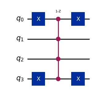
• a. $|0000\rangle$
• b. $|0101\rangle$
• c. $|0110\rangle$
• d. $|1001\rangle$
• e. $|1010\rangle$
• f. $|1111\rangle$

3. Suppose you want to search for three marked states from a set of 128. What is the optimal number of iterations of the Grover operator to maximize the amplitudes of the marked states?

• a. 1
• b. 3
• c. 5
• d. 6
• e. 20
• f. 33

Discussion questions:

1. What other problems could you formulate as a Grover search? Think of problems where it is difficult to find a solution but easy to verify one.

2. Can you see any problems with scaling Grover's algorithm on modern quantum computers?