Ground-state energy estimation of the Heisenberg chain with VQE

Usage estimate: 37 minutes on a Heron processor (NOTE: This is an estimate only. Your runtime might vary.)

Learning outcomes

After completing this tutorial, you can expect to understand the following information:

• How to model a Heisenberg spin chain as a quantum Hamiltonian using Qiskit
• How to use the SPSA optimizer to estimate the ground-state energy of a quantum system
• How to execute variational workflows on IBM® quantum hardware using Qiskit Runtime primitives and sessions

Prerequisites

It is recommended that you familiarize yourself with these topics:

• Basics of quantum information
• Introduction to Qiskit patterns
• Variational algorithm design

Background

The Heisenberg spin chain is one of the most widely studied models in condensed matter physics and quantum magnetism. It describes a one-dimensional lattice of interacting quantum spins, where nearest-neighbor spins are coupled through exchange interactions. The Hamiltonian for the isotropic Heisenberg model with an external magnetic field is given by:

$H = \sum_{\langle i,j \rangle} \left( J_x X_i X_j + J_y Y_i Y_j + J_z Z_i Z_j \right) + \sum_{i} h_i Z_i,$

where $X_i$, $Y_i$, and $Z_i$ are the Pauli operators acting on site $i$, the sum $\langle i,j \rangle$ runs over nearest-neighbor pairs, $J_x = J_y = J_z = 0.5$ are the exchange coupling constants (isotropic in this tutorial), and $h_i$ represents a site-dependent external magnetic field. In this tutorial, the magnetic field values are randomly sampled from the interval $[-1, 1]$. Note that in the implementation below, the set of "nearest-neighbor" pairs is determined by the hardware backend's native coupling among the first $N$ qubits, which might not form a strict linear chain depending on the device topology.

Understanding the ground-state energy of this Hamiltonian is of fundamental importance in physics. The ground state encodes information about quantum phase transitions, entanglement structure, and magnetic ordering. Classically, computing the exact ground-state energy becomes intractable as the number of spins grows, since the Hilbert space dimension scales exponentially as $2^N$ for $N$ spins. This makes it a natural candidate for quantum simulation.

The Variational Quantum Eigensolver (VQE) is a hybrid quantum-classical algorithm designed to estimate the ground-state energy of a Hamiltonian. It works by preparing a parameterized quantum state $|\psi(\theta)\rangle$ (called an ansatz) on a quantum computer and measuring the expectation value $\langle \psi(\theta) | H | \psi(\theta) \rangle$. A classical optimizer then iteratively adjusts the parameters $\theta$ to minimize this energy, leveraging the variational principle which guarantees that the measured energy is always an upper bound to the true ground-state energy.

In this tutorial, we use the efficient_su2 ansatz from Qiskit's circuit library, which constructs layers of single-qubit rotations and entangling gates. The optimization is carried out using the Simultaneous Perturbation Stochastic Approximation (SPSA) algorithm, which is well-suited for noisy quantum hardware because it estimates gradients using only two function evaluations per iteration regardless of the number of parameters.

Requirements

Before starting this tutorial, ensure that you have the following installed:

• Qiskit SDK v2.0 or later, with visualization support
• Qiskit Runtime v0.44 or later (pip install qiskit-ibm-runtime)

Setup

import numpy as np
import matplotlib.pyplot as plt
from typing import Sequence

from qiskit import QuantumCircuit
from qiskit.quantum_info import SparsePauliOp
from qiskit.primitives import BaseEstimatorV2
from qiskit.circuit.library import XGate
from qiskit.circuit.library import efficient_su2
from qiskit.transpiler import PassManager
from qiskit.transpiler.preset_passmanagers import generate_preset_pass_manager
from qiskit.transpiler.passes.scheduling import (
    ALAPScheduleAnalysis,
    PadDynamicalDecoupling,
)
from qiskit_ibm_runtime import QiskitRuntimeService, Session, EstimatorV2


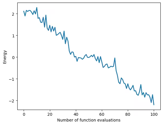
def visualize_results(results):
    plt.plot(results["cost_history"], lw=2)
    plt.xlabel("Number of function evaluations")
    plt.ylabel("Energy")
    plt.show()

Small-scale example

In this section, we walk through each step of the Qiskit pattern at a small scale, explaining the key components as we build up the workflow.

Step 1: Map classical inputs to a quantum problem

• Input: Number of spins
• Output: Ansatz and Hamiltonian modeling the Heisenberg chain

Construct an ansatz and Hamiltonian that model a 10-spin Heisenberg chain. In this step, we will build a 10-spin Heisenberg Hamiltonian over the least-busy backend's coupling map and prepare the efficient_su2 ansatz.

num_spins = 10
ansatz = efficient_su2(num_qubits=num_spins, reps=2)

service = QiskitRuntimeService()
backend = service.least_busy(
    operational=True, min_num_qubits=num_spins, simulator=False
)

coupling = backend.target.build_coupling_map()
reduced_coupling = coupling.reduce(list(range(num_spins)))

edge_list = reduced_coupling.graph.edge_list()
ham_list = []

for edge in edge_list:
    ham_list.append(("ZZ", edge, 0.5))
    ham_list.append(("YY", edge, 0.5))
    ham_list.append(("XX", edge, 0.5))

for qubit in reduced_coupling.physical_qubits:
    ham_list.append(("Z", [qubit], np.random.random() * 2 - 1))

hamiltonian = SparsePauliOp.from_sparse_list(ham_list, num_qubits=num_spins)

ansatz.draw("mpl", style="iqp")

Output:

Step 2: Optimize problem for quantum hardware execution

• Input: Abstract circuit, observable
• Output: Target circuit and observable, optimized for the selected QPU

Use the generate_preset_pass_manager function from Qiskit to automatically generate an optimization routine for our circuit with respect to the selected QPU. We choose optimization_level=3, which provides the highest level of optimization of the preset pass managers. We also include ALAPScheduleAnalysis and PadDynamicalDecoupling scheduling passes to suppress decoherence errors.

target = backend.target
pm = generate_preset_pass_manager(optimization_level=3, target=target)
pm.scheduling = PassManager(
    [
        ALAPScheduleAnalysis(durations=target.durations()),
        PadDynamicalDecoupling(
            durations=target.durations(),
            dd_sequence=[XGate(), XGate()],
            pulse_alignment=target.pulse_alignment,
        ),
    ]
)
isa_ansatz = pm.run(ansatz)
isa_observable = hamiltonian.apply_layout(isa_ansatz.layout)
isa_ansatz.draw("mpl", scale=0.6, style="iqp", fold=-1, idle_wires=False)

Output:

Step 3: Execute using Qiskit primitives

• Input: Target circuit and observable
• Output: Results of optimization

Minimize the estimated ground-state energy of the system by optimizing the circuit parameters. Use the Estimator primitive from Qiskit Runtime to evaluate the cost function during optimization.

Since we optimized the circuit for the backend in Step 2, we can avoid doing transpilation on the Runtime server by setting skip_transpilation=True and passing the optimized circuit. For this demo, we will run on a QPU using qiskit-ibm-runtime primitives. To run with qiskit statevector-based primitives, replace the block of code using Qiskit Runtime primitives with the commented block.

In this tutorial we use Simultaneous Perturbation Stochastic Approximation (SPSA), which is a gradient-based optimizer. Next we give a brief introduction to it, and provide the code to implement SPSA using Qiskit v2.0.

Introducing SPSA

Simultaneous Perturbation Stochastic Approximation (SPSA) [1] is an optimization algorithm that approximates the entire gradient vector using only two function calls at each iteration. Let $f:\mathbb{R}^p\rightarrow \mathbb{R}$ be the cost function with $p$ parameters to be optimized, and $x_i\in \mathbb{R}^p$ be the parameter vector at the $i^{th}$ step of the iteration. To compute the gradient, a random vector $\Delta_i$ of size $p$ is created, where each element $\Delta_{ij}$, $\forall$ $j\in \{1,2,...,p\}$, is uniformly sampled from $\{-1, 1\}$. Next, each element of the random vector $\Delta_i$ is multiplied with a small value $c_i$ to create a random perturbation. The gradient is then estimated as

$[\nabla f(x_i)]_j \approx \frac{f(x_i + c_i \Delta_i) - f(x_i - c_i \Delta_i)}{2c_i\Delta_{ij}}.$

Intuitively, since a random perturbation is applied during the gradient estimation, it is expected that small deviations in the exact values of $f$ coming from noise can be tolerated and accounted for. In fact, SPSA is particularly known to be robust against noise, and requires only two hardware calls for each iteration. It is, therefore, one of the highly preferred optimizers for implementing variational algorithms.

In this tutorial, the hyperparameters for the $i^{th}$ iteration, $a_i$ and $c_i$, are computed as

$a_i = \frac{a}{(A + i + 1)^\alpha} \quad \text{and} \quad c_i = \frac{c}{(i+1)^\gamma},$

where the constant values are taken as $A = 30$, $\alpha = 0.9$, $a = 0.3$, $c = 0.1$, and $\gamma = 0.4$. These values are selected from [2]. Appropriate tuning of hyperparameters is necessary for extracting a good performance out of SPSA.

def spsa(
    fun, x0, args=(), A=30, alpha=0.9, a=0.3, c=0.1, gamma=0.4, maxiter=100
):
    nparams = len(x0)
    x = np.copy(x0)

    for i in range(maxiter):
        a_i = a / (A + i + 1) ** alpha
        c_i = c / (i + 1) ** gamma
        delta_i = np.random.choice([-1, 1], nparams)

        # two hardware calls
        eval_1 = fun(x + c_i * delta_i, *args)
        eval_2 = fun(x - c_i * delta_i, *args)

        # compute the gradient and update the parameters
        grad = (eval_1 - eval_2) / (2 * c_i) * np.reciprocal(delta_i)
        x = x - a_i * grad

    return x

def cost_func(
    params: Sequence,
    ansatz: QuantumCircuit,
    hamiltonian: SparsePauliOp,
    estimator: BaseEstimatorV2,
    cost_history_dict: dict,
) -> float:
    """Ground state energy evaluation."""
    energy = (
        estimator.run([(ansatz, hamiltonian, [params])]).result()[0].data.evs
    )

    cost_history_dict["iters"] += 1
    cost_history_dict["prev_vector"] = list(params)
    cost_history_dict["cost_history"].append(float(energy[0]))

    print(
        f"Fx Iters. done: {cost_history_dict['iters']} [Current cost: {round(energy[0], 5)}]",
        end="\r",
    )

    return energy


def solve(x0, isa_ansatz, isa_observable, maxiter=150):
    cost_history_dict = {
        "prev_vector": None,
        "iters": 0,
        "cost_history": [],
        "y_min": None,
    }

    # Evaluate the problem using a QPU via Qiskit IBM Runtime
    with Session(backend=backend) as session:
        estimator = EstimatorV2(mode=session)
        estimator.skip_transpilation = True
        estimator.options.environment.job_tags = ["TUT_HSVQE"]
        x_opt = spsa(
            cost_func,
            x0=x0,
            args=(isa_ansatz, isa_observable, estimator, cost_history_dict),
            maxiter=maxiter,
        )

        y_min = cost_func(
            x_opt, isa_ansatz, isa_observable, estimator, cost_history_dict
        )

    return y_min, cost_history_dict

np.random.seed(42)
num_params = ansatz.num_parameters
params = 2 * np.pi * np.random.random(num_params)

Here we set the maxiter = 50. Note that since each iteration requires two calls to the function to compute the gradient, the total number of function calls will be $2 \times \text{maxiter}$. The maxiter can be increased to any higher value for better energy estimation.

maxiter = 50
spsa_min, spsa_history = solve(
    params, isa_ansatz, isa_observable, maxiter=maxiter
)

Output:

Fx Iters. done: 101 [Current cost: -3.03843]

Step 4: Post-process and return result in desired classical format

• Input: Ground-state energy estimates during optimization
• Output: Estimated ground-state energy

print(f"Estimated ground state energy: {spsa_min}")

Output:

Estimated ground state energy: [-3.03842968]

results = {
    "spsa": spsa_history,
}

visualize_results(spsa_history)

Output:

Large-scale hardware example

A large-scale hardware example is not included in this tutorial. As the number of qubits increases, VQE encounters significant challenges due to the barren plateau phenomenon: the gradient of the cost function vanishes exponentially with system size, making optimization practically infeasible for large circuits. Combined with hardware noise, this means that scaling VQE to larger spin chains does not produce reliably reproducible results. For approaches that overcome these limitations, see the Next Steps section below.

Challenge

Now that you have a working VQE implementation for the Heisenberg chain, try the following:

1. Experiment with ansatz depth: Modify the reps parameter in efficient_su2 (for example, try reps=1 and reps=3). How does ansatz depth affect the estimated ground-state energy and convergence speed? At what point do you observe diminishing returns or instability?
2. Tune SPSA hyperparameters: Adjust the learning rate schedule parameters (a, c, alpha, gamma, A) and observe how they impact convergence. Can you find a configuration that converges faster than the defaults used here?
3. Compare coupling topologies: Instead of using the backend's native coupling map, try constructing a simple nearest-neighbor linear chain and compare the results. How does the connectivity of the physical hardware affect the transpiled circuit depth and final energy estimate?

References

[1] Spall, J. C. (2002). Implementation of the simultaneous perturbation algorithm for stochastic optimization. IEEE Transactions on Aerospace and Electronic Systems, 34(3), 817-823.

[2] Sahin, M. Emre, et al. (2025). Qiskit Machine Learning: an open-source library for quantum machine learning tasks at scale on quantum hardware and classical simulators. arXiv:2505.17756.

Next steps