Quantum kernel training

Usage estimate: under one minute on a Heron r3 processor (NOTE: This is an estimate only. Your runtime might vary.)

Learning outcomes

After completing this tutorial, you can expect to understand the following information:

• Kernel methods and their uses
• Quantum kernels and how they can provide enhanced feature spaces
• Quantum kernel circuit construction
• How to train a quantum kernel using a Qiskit pattern: map, optimize, execute, and post-process

Prerequisites

It is recommended that you familiarize yourself with quantum kernels, why they are important, and how they are used in practice.

• Covariant quantum kernels for data with group structure (paper)
• Introduction to Quantum Kernels and Support Vector Machines (video)
• Quantum Kernels in Practice (video)

It is also useful to have a basic understanding of group theory.

Background

Kernel methods are commonplace in machine learning applications. In this context, "kernel" refers to the kernel matrix or individual entries therein. In general, a kernel is a similarity measure between data encoded in a high-dimensional feature space and can be utilized, for example, in classification tasks with support vector machines.

Quantum kernel methods are those which use quantum computers to estimate a kernel. It is known that quantum computers can encode data in quantum-enhanced feature spaces, effectively replacing classical analogs. For $\vec{x} \in \mathbb{R}$ and $\Psi(\vec{x}) \in \mathbb{R}^{d'}$, typically with $d' >d$, $\Psi(\vec{x})$ is a feature map, $\vec{x} \mapsto \Psi(\vec{x})$. The goal of $\Psi(\vec{x})$ is to make categories of data separated by a hyperplane. Taking the vectors in the feature-mapped space as arguments, kernel function $K(\vec{x}, \vec{y}) = \langle{\Psi(\vec{x}) | \Psi(\vec{y}) \rangle{}}$ returns their inner product: $K: \mathbb{R}^d \rightarrow$ $\mathbb{R}^d$. Classically, feature maps of interest are those in which the kernel function can be easily evaluated; as in, when the inner product in the feature-mapped space can be written in terms of the original data vectors and $\Psi(\vec{x})$ and $\Psi(\vec{y})$ do not need to be constructed. In the case of quantum kernels, feature mapping is performed by a quantum circuit, and the kernel is estimated using the measurement probabilities sampled from the circuit.

This tutorial shows how to build a Qiskit pattern for evaluating entries into a quantum kernel matrix used for binary classification.

Requirements

Before starting this tutorial, be sure you have the following installed:

• Qiskit SDK v2.3.1 or later, with visualization support
• Qiskit Runtime v0.44.0 or later (pip install qiskit-ibm-runtime)

Setup

# General Imports and helper functions
import urllib.request

import pandas as pd
import numpy as np
import matplotlib.pyplot as plt


from qiskit.circuit import Parameter, ParameterVector, QuantumCircuit
from qiskit.circuit.library import unitary_overlap
from qiskit.primitives import StatevectorSampler
from qiskit.transpiler.preset_passmanagers import generate_preset_pass_manager

from qiskit_ibm_runtime import QiskitRuntimeService, Sampler

# Download the dataset (portable across platforms)
urllib.request.urlretrieve(
    "https://raw.githubusercontent.com/qiskit-community/prototype-quantum-kernel-training/main/data/dataset_graph7.csv",
    "dataset_graph7.csv",
)


def visualize_counts(res_counts, num_qubits, num_shots):
    """Visualize the outputs from the Qiskit Sampler primitive."""
    zero_prob = res_counts.get(0, 0.0)
    top_10 = dict(
        sorted(res_counts.items(), key=lambda item: item[1], reverse=True)[
            :10
        ]
    )
    top_10.update({0: zero_prob})
    by_key = dict(sorted(top_10.items(), key=lambda item: item[0]))
    x_vals, y_vals = list(zip(*by_key.items()))
    x_vals = [bin(x_val)[2:].zfill(num_qubits) for x_val in x_vals]
    y_vals_prob = []
    for t in range(len(y_vals)):
        y_vals_prob.append(y_vals[t] / num_shots)
    y_vals = y_vals_prob
    plt.bar(x_vals, y_vals)
    plt.xticks(rotation=75)
    plt.title("Results of sampling")
    plt.xlabel("Measured bitstring")
    plt.ylabel("Probability")
    plt.show()


def get_training_data():
    """Read the training data."""
    df = pd.read_csv("dataset_graph7.csv", sep=",", header=None)
    training_data = df.values[:20, :]
    ind = np.argsort(training_data[:, -1])
    X_train = training_data[ind][:, :-1]

    return X_train

Small-scale simulator example

In this section, we walk through the four steps of the Qiskit pattern on a seven-qubit instance of the labeling-cosets-with-error problem and evaluate a single kernel matrix entry using the StatevectorSampler primitive from Qiskit. A statevector simulator is exact (up to shot noise) and shows us the method end-to-end without consuming QPU time. We then repeat the same instance on real hardware in the hardware example section.

Step 1: Map classical inputs to a quantum problem

• Input: Training dataset.
• Output: Abstract circuit for calculating a kernel matrix entry.

The binary classification problem we aim to solve here is referred to as "labeling cosets with error." The input training dataset contains a group structure, consisting of two cosets formed by a group and subgroup. The group is taken to be $G = SU(2)^{\otimes n}$ for qubits, which is the special unitary group of $2 \times 2$ matrices and has wide applicability in nature; e.g., the Standard Model of particle physics. We take the (graph-stabilizer) subgroup $S_\text{graph} < G$ with $S_\text{graph} = \langle \{ X_i \otimes _{k:(k,i) \in \mathcal{E}} Z_k\} _{i \in \mathcal{V}} \} \rangle$ for a graph with edges $\mathcal{E}$ and vertices $\mathcal{V}$. Note that the stabilizers fix a stabilizer state such that $D_s | \psi \rangle = | \psi \rangle,~ \forall s \in S_\text{graph}$. Finally, we define two left-cosets $C_\pm = c_\pm S_\text{graph}$ by drawing two $c_\pm \in G$ at random.

For more details about the dataset and how it is generated, see this notebook from the Quantum Kernel Training Toolkit.

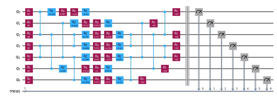
We create the quantum circuit used to evaluate one entry in the kernel matrix. The input data is used to determine the rotation angles for the circuit's parametrized gates. For simplicity, we will use data samples x1=14 and x2=19.

Note: The dataset used in this tutorial can be downloaded here.

# Prepare training data
X_train = get_training_data()

# Empty kernel matrix
num_samples = np.shape(X_train)[0]
kernel_matrix = np.full((num_samples, num_samples), np.nan)

# Prepare feature map for computing overlap
num_features = np.shape(X_train)[1]
num_qubits = int(num_features / 2)
entangler_map = [[0, 2], [3, 4], [2, 5], [1, 4], [2, 3], [4, 6]]
fm = QuantumCircuit(num_qubits)
training_param = Parameter("θ")
feature_params = ParameterVector("x", num_qubits * 2)
fm.ry(training_param, fm.qubits)
for cz in entangler_map:
    fm.cz(cz[0], cz[1])
for i in range(num_qubits):
    fm.rz(-2 * feature_params[2 * i + 1], i)
    fm.rx(-2 * feature_params[2 * i], i)

# Assign tunable parameter to known optimal value and set the data params for first two samples
x1 = 14
x2 = 19
unitary1 = fm.assign_parameters(list(X_train[x1]) + [np.pi / 2])
unitary2 = fm.assign_parameters(list(X_train[x2]) + [np.pi / 2])

# Create the overlap circuit
overlap_circ = unitary_overlap(unitary1, unitary2)
overlap_circ.measure_all()
overlap_circ.draw("mpl", scale=0.6, style="iqp")

Output:

Step 2: Optimize problem for quantum hardware execution

• Input: Abstract circuit, not optimized for a particular backend.
• Output: Target circuit, optimized for the selected QPU.

For the statevector simulator path used in this section, no backend-specific optimization is required: the abstract circuit can be sampled directly. We exercise this step in the hardware example below, where the circuit is transpiled against a real QPU using generate_preset_pass_manager with optimization_level=3.

Step 3: Execute using Qiskit primitives

• Input: Abstract circuit.
• Output: Quasi-probability distribution.

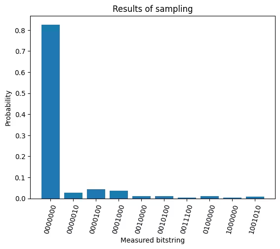
Use the StatevectorSampler primitive from Qiskit to reconstruct a quasi-probability distribution of states yielded from sampling the circuit. For the task of generating a kernel matrix, we are particularly interested in the probability of measuring the |0> state.

sampler = StatevectorSampler()

# Execute and get counts
num_shots = 10_000
results = sampler.run([overlap_circ], shots=num_shots).result()
counts = results[0].data.meas.get_int_counts()

# Plot counts
visualize_counts(counts, num_qubits, num_shots)

Output:

Step 4: Post-process and return result in desired classical format

• Input: Probability distribution.
• Output: A single kernel matrix element.

Calculate the probability of measuring $|0 \rangle$ on the overlap circuit, and populate the kernel matrix in the position corresponding to the samples represented by this particular overlap circuit (row 15, column 20).

kernel_matrix[x1, x2] = counts.get(0, 0.0) / num_shots
print(f"Fidelity (simulator): {kernel_matrix[x1, x2]}")

Output:

Fidelity (simulator): 0.8261

Hardware example

A quantum kernel matrix has $\mathcal{O}(N^2)$ entries for $N$ training samples, and each entry requires running an overlap circuit whose two-qubit-gate depth grows with the size of the feature map. As a result, scaling this tutorial to a larger problem has two compounding costs: the QPU time per kernel matrix grows quadratically with $N$, and the depth of unitary_overlap (which composes the feature map with its adjoint) erodes fidelity at the system size and connectivity of current hardware. To keep the demo short and to make a clean comparison, we therefore run the same seven-qubit instance from the small-scale example on a real QPU and compare the fidelity of a single kernel matrix entry against the simulator value computed above.

# ------------------------------ Step 1 ------------------------------
# Prepare training data
X_train = get_training_data()

# Empty kernel matrix
num_samples = np.shape(X_train)[0]
kernel_matrix = np.full((num_samples, num_samples), np.nan)

# Prepare feature map for computing overlap
num_features = np.shape(X_train)[1]
num_qubits = int(num_features / 2)
entangler_map = [[0, 2], [3, 4], [2, 5], [1, 4], [2, 3], [4, 6]]
fm = QuantumCircuit(num_qubits)
training_param = Parameter("θ")
feature_params = ParameterVector("x", num_qubits * 2)
fm.ry(training_param, fm.qubits)
for cz in entangler_map:
    fm.cz(cz[0], cz[1])
for i in range(num_qubits):
    fm.rz(-2 * feature_params[2 * i + 1], i)
    fm.rx(-2 * feature_params[2 * i], i)

# Assign tunable parameter to known optimal value and set the data params for first two samples
x1 = 14
x2 = 19
unitary1 = fm.assign_parameters(list(X_train[x1]) + [np.pi / 2])
unitary2 = fm.assign_parameters(list(X_train[x2]) + [np.pi / 2])

# Create the overlap circuit
overlap_circ = unitary_overlap(unitary1, unitary2)
overlap_circ.measure_all()

# ------------------------------ Step 2 ------------------------------
service = QiskitRuntimeService()
# backend = service.least_busy(
#    operational=True, simulator=False, min_num_qubits=overlap_circ.num_qubits
# )
backend = service.backend("ibm_pittsburgh")
print(f"Using backend: {backend.name}")
pm = generate_preset_pass_manager(optimization_level=3, backend=backend)
overlap_ibm = pm.run(overlap_circ)

# ------------------------------ Step 3 ------------------------------
sampler = Sampler(mode=backend)
sampler.options.environment.job_tags = ["TUT_QKT"]

num_shots = 10_000
results = sampler.run([overlap_ibm], shots=num_shots).result()
counts = results[0].data.meas.get_int_counts()
visualize_counts(counts, num_qubits, num_shots)

# ------------------------------ Step 4 ------------------------------
kernel_matrix[x1, x2] = counts.get(0, 0.0) / num_shots
print(f"Fidelity (hardware): {kernel_matrix[x1, x2]}")

Output:

Using backend: ibm_pittsburgh

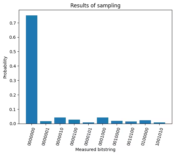
Fidelity (hardware): 0.7517

To fill out the entire kernel matrix, we would run a quantum experiment for each of its $N(N+1)/2$ unique entries. The figure below shows the resulting matrix for this dataset; darker red indicates fidelities closer to 1.0.

Next steps