HI-VQE Chemistry - A Qiskit Function by Qunova Computing
See the API reference
Qiskit Functions are an experimental feature available only to IBM Quantum® Premium Plan, Flex Plan, and On-Prem (via IBM Quantum Platform API) Plan users. They are in preview release status and subject to change.
The code on this page was developed using the following requirements. We recommend using these versions or newer.
qiskit-ibm-runtime~=0.45.0
Overview
In quantum chemistry, the electronic structure problem focuses on finding the solutions to the electronic Schrödinger equation - the quantum wave functions describing the behavior of the system's electrons. These wave functions are vectors of complex amplitudes, with each amplitude corresponding to the contribution of a possible electron configuration.
The ground state is the lowest energy wave function of the system and has a special importance in the study of molecular systems. The most accurate approach for computing the ground state considers all possible electron configurations, but this becomes intractable for larger systems since the number of configurations grows exponentially with system size.
The Handover Iterative Variational Quantum Eigensolver (HI-VQE) is an innovative hybrid quantum-classical method for accurately estimating the ground state of molecular systems. It integrates quantum hardware with classical computing, using quantum processors to efficiently explore candidate electron configurations and calculating the resulting wave function on classical computers. By generating compact yet chemically accurate wave functions, HI-VQE enhances research and discovery in quantum chemistry and materials science.


HI-VQE reduces the computational complexity of the electronic structure problem by efficiently estimating the ground state with high accuracy. It focuses on a carefully selected subset of the most relevant electron configurations, optimizing both accuracy and efficiency.
Combining the strengths of both classical and quantum computers, HI-VQE iteratively refines and improves the current estimate wave function. Its unique subspace construction techniques help make configuration selection more efficient, so that users have greater computational control and improved accuracy in quantum chemistry simulations.
If you would like to learn about the algorithm in more depth, you can read the associated research paper
Description
The number of electron configurations for a molecular system grows exponentially with system size. However, for certain electronic states, such as the ground state, it is common that only a small fraction of configurations significantly contribute to the state’s energy. Selected configuration interaction (SCI) methods exploit this sparsity to reduce computational costs by identifying and focusing on the most relevant configurations. This subset of configurations is referred to as a subspace.
HI-VQE leverages the inherent efficiency of quantum computers for representing molecular systems to aid the subspace search. It integrates classical and quantum subroutines to solve the electronic structure problem with high accuracy. Unlike existing quantum SCI methods, HI-VQE combines variational training, iterative subspace construction, and pre-diagonalization configuration screening to enhance efficiency by reducing quantum measurements, iterations, and classical diagonalization costs. HI-VQE can therefore be applied to larger molecular systems which require more qubits, and reduces the cost to solve a problem of a given size to the same degree of accuracy.
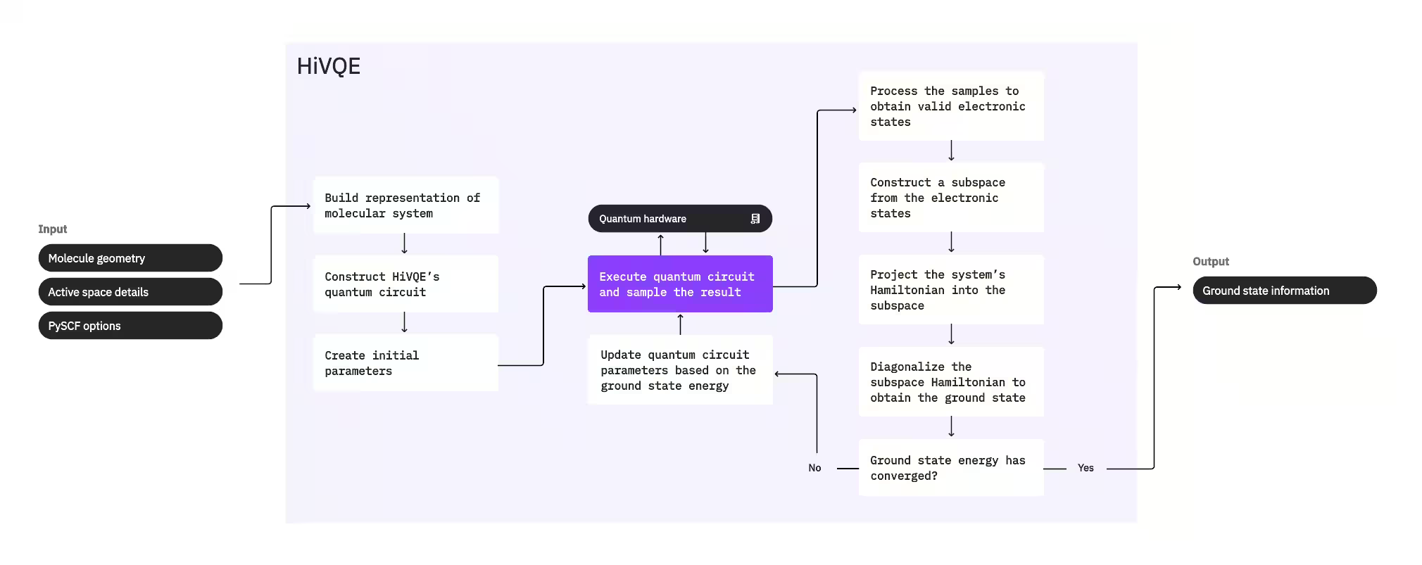

To compute a system's ground state, HI-VQE first uses the classical chemistry package PySCF to generate a molecular representation from user-provided inputs, such as the molecular geometry and other molecular information. It then enters a hybrid quantum-classical optimization loop, iteratively refining a subspace to optimally represent the ground state while minimizing the number of configurations included. The loop continues until convergence criteria, such as subspace size or energy stability, are met, after which the computed ground state wave function and energy are output. These results can be used to construct accurate potential energy surfaces and perform further analysis of the system.
The optimization loop focuses on adjusting a quantum circuit’s parameters to generate a high-quality subspace. HI-VQE offers three quantum circuit options: excitation_preserving, efficient_su2, and LUCJ. The optimization is initialized close to the Hartree-Fock reference state due to its general suitability. The circuit is then executed on a quantum device and configurations are sampled from the resulting quantum state before being returned as binary strings. Due to quantum device noise, some sampled configurations may be physically invalid, failing to conserve electron number or spin. HI-VQE addresses this using the configuration recovery process from the qiskit-addon-sqd package, so that users can either correct invalid configurations or discard them.
The valid configurations then undergo an optional screening step to remove those predicted to contribute minimally. This reduces the dimension of the subspace, thereby lowering the cost of the diagonalization step. If the screening is enabled, then a preliminary subspace Hamiltonian is constructed from the valid configurations and a diagonalization is performed with very loose termination critieria. Though the accuracy of the resulting amplitudes for each configuration is low, it is effective for predicting which configurations to leave out of the subspace this iteration, and it is fast to compute.
The selected configurations are added to the subspace, and the system's Hamiltonian is projected into this subspace. The subspace updates iteratively, preserving the most relevant configurations across iterations. This approach contrasts with alternative methods because the quantum circuit does not need to approximate the full ground state at each step.
Next, the subspace Hamiltonian is classically diagonalized to obtain the lowest eigenvalue and its corresponding eigenvector, representing an approximation of the ground state and its energy. As the subspace quality improves through iterations, the computed ground state better approximates the true ground state. An additional screening step can be performed at this point to remove any configurations from the subspace that don't have a substantial contribution to the computed ground state. This step ensures that the subspace carried into the next iteration is as compact as possible. This is evaluated based on the amplitudes that are returned by the diagonalization, as these represent each configuration's importance contribution to the computed ground state.
A convergence check then determines whether further training would improve results. If so, then an optional classical expansion step is performed, the quantum circuit parameters are updated to further minimize the computed energy, and the process repeats. The classical expansion step generates additional configurations for the subspace, supplementing the configurations sampled from the quantum device. It first identifies the configuration with the largest amplitude in the diagonalization results, before generating new configurations with single and double excitations from the identified configuration. The desired number of these configurations are then added to the subspace.
Once it is determined that the iterations have converged, HI-VQE returns the computed ground state (in the form of the states in the subspace and their amplitudes in the ground state wave function), its energy, and an energy variance measure that gives an indication of whether the computed state forms an eigenstate of the system's Hamiltonian.
Users are able to decide the quantum circuit used and the number of shots taken for each quantum circuit, as well as control the subspace size or enable the classical generation of additional configurations to assist the quantum generated configurations. In this way users can tailor the behavior of HI-VQE to suit their desired applications.
Licensing
Please note that use of this Qiskit Function is limited to problems requiring at most 20 qubits, unless a license is obtained granting a higher limit.
Please email qiskit.support@qunovacomputing.com if you would like to inquire about obtaining a license.
Get started
First, request access to the function. Then, authenticate using your IBM Quantum® API key and, assuming you've already saved your account to your local environment, select the Qiskit Function as follows:
import reprlib
from qiskit_ibm_catalog import QiskitFunctionsCatalog

catalog = QiskitFunctionsCatalog(channel="ibm_quantum_platform")

# Verify that you have access to the function
catalog.list()
Output:
[QiskitFunction(qunova/hivqe-chemistry),
 QiskitFunction(global-data-quantum/quantum-portfolio-optimizer),
 QiskitFunction(algorithmiq/tem),
 QiskitFunction(qedma/qesem),
 QiskitFunction(multiverse/singularity),
 QiskitFunction(ibm/circuit-function),
 QiskitFunction(q-ctrl/optimization-solver),
 QiskitFunction(colibritd/quick-pde),
 QiskitFunction(q-ctrl/performance-management),
 QiskitFunction(kipu-quantum/iskay-quantum-optimizer)]
# Load the function
function = catalog.load("qunova/hivqe-chemistry")
Example
The first example shows how to compute the ground state energy for an NH3 molecule using the HI-VQE algorithm.
Define the molecular geometry and options
The molecular geometry of NH3 is provided with Cartesian coordinates separated with ";" for each atom.
# Define the molecule geometry
geometry = """
N         -0.85188       -0.02741        0.03141;
H          0.16545        0.00593       -0.01648;
H         -1.16348       -0.39357       -0.86702;
H         -1.16348        0.94228        0.06281;
"""
Additional options can be defined and provided for molecular system in the following dictionary format.
# Configure some options for the job.
molecule_options = {"basis": "sto3g"}
hivqe_options = {"shots": 100, "max_iter": 20}
Execute the function with geometry and option inputs.
# Run HI-VQE
job = function.run(
    geometry=geometry,
    # `backend_name` is the name of a backend with at least 16 qubits,
    # for example, "ibm_marrakesh".
    backend_name=backend_name,
    max_states=2000,
    max_expansion_states=10,
    molecule_options=molecule_options,
    hivqe_options=hivqe_options,
)
It is a good idea to print the Function job ID so that it can be provided in support requests if something goes wrong.
print("Job ID:", job.job_id)Output:
Job ID: e5ced6f2-fd1d-4244-a6aa-bd27cfb0cdee
This example then utilizes 16 qubits with 8 orbitals of sto3g basis for an NH3 molecule.
Check your Qiskit Function workload's status or return results as follows:
print(job.status())Output:
QUEUED
After the job is completed, the results can be obtained with result() instance.
result = job.result()

# Output can be long, so we display a shortened representation
shortened_result = reprlib.repr(result)
print(shortened_result)
Output:
{'eigenvector': [0.9824448589364075, 0.009527106392132133, 6.854074372058527e-08, 3.591500190038039e-07, 0.0012975231577544268, 2.310159709002111e-05, ...], 'energy': -55.52108557170985, 'energy_history': [-55.51901898989887, -55.52056881448526, -55.52065046778772, -55.520690696813716, -55.520691108428, -55.520708448092634, ...], 'energy_variance': 3.066239097617371e-10, ...}
To access the ground state energy, use the "energy" key. The "eigenvector" key provides the CI coefficients with corresponding bitstring notation of electron configuration stored with "states" of the results.
fci_energy = -55.521148034704126  # the exact energy using FCI method
hivqe_energy = result["energy"]
print(
    f"|Exact Energy - HI-VQE Energy|: "
    f"{abs(fci_energy - hivqe_energy) * 1000} mHa"
)
print(f"Sampled Number of States: {len(result['states'])}")
Output:
|Exact Energy - HI-VQE Energy|: 0.06246299427914437 mHa
Sampled Number of States: 1936
Performance
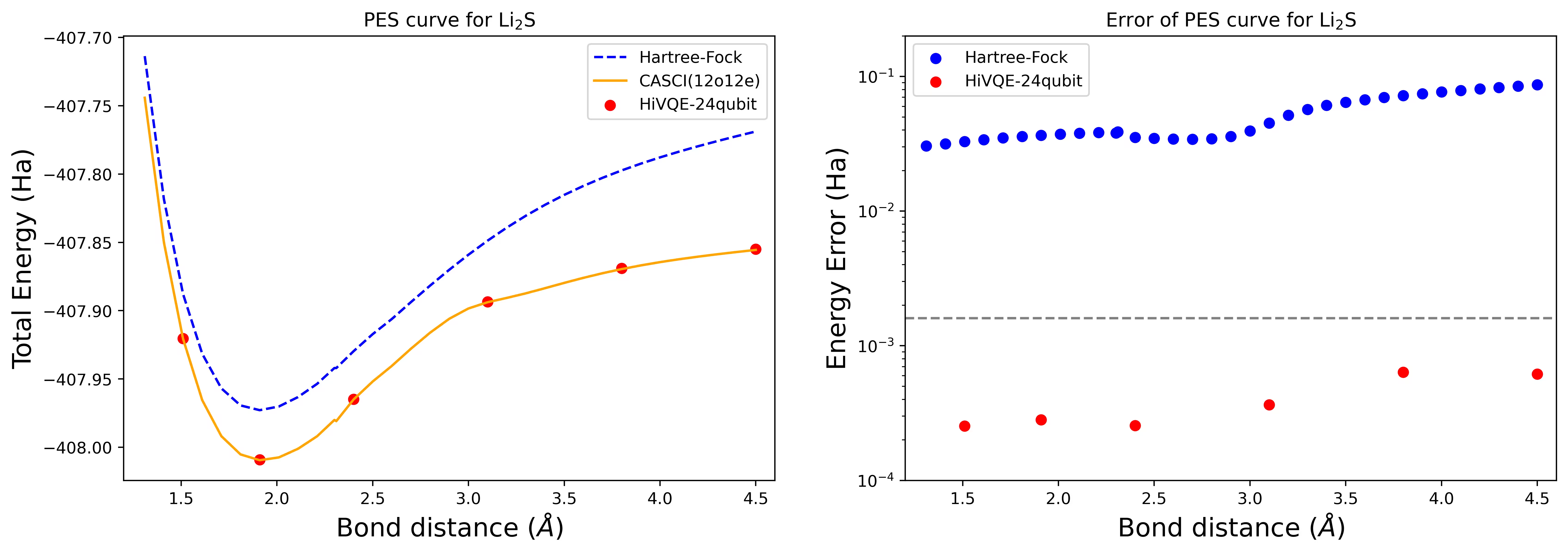
This section shows the demonstrated benchmark calculations of HI-VQE with a 24-qubit case for Li2S, a 40-qubit case for an N2 molecule, and a 44-qubit case for an FeP-NO system.
Dissociation potential energy surface curve for an Li2S molecule with 24 qubits
The PES curve is shown with the FCI reference and initial guess from RHF, together with the energy error from the FCI reference.
 .
.
The calculations have been conducted with the following geometries and options.
# Define Li2S geometries
Li2S_geoms = {
    "Li2S_1.51": "S        -1.239044    0.671232   -0.030374;Li       -1.506327    0.432403   -1.498949;Li       -0.899996    0.973348    1.826768;",
    "Li2S_2.40": "S        -1.741432    0.680397    0.346702;Li       -0.529307    0.488006   -1.729343;Li       -1.284307    0.989409    2.177209;",
    "Li2S_3.80": "S        -2.707255    0.674298    0.909161;Li        0.079218    0.552012   -1.671656;Li       -0.927010    0.931502    1.557063;",
}

# Configure some options for the job.
molecule_options = {
    "basis": "sto3g",
}
hivqe_options = {
    "shots": 100,
    "max_iter": 20,
}

results = []
for geom in ["Li2S_1.51", "Li2S_2.40", "Li2S_3.80"]:
    # Run HI-VQE
    job = function.run(
        geometry=Li2S_geoms[geom],
        backend_name=backend_name,  # can use any device with at least 38 qubits
        max_states=2000,
        max_expansion_states=10,
        molecule_options=molecule_options,
        hivqe_options=hivqe_options,
    )
    results.append(job.result())
The red dots represent the HI-VQE calculation results for six different geometries, and three geometries corresponding to 1.51, 2.40, and 3.80 Angstrom are provided as input in the above cell.
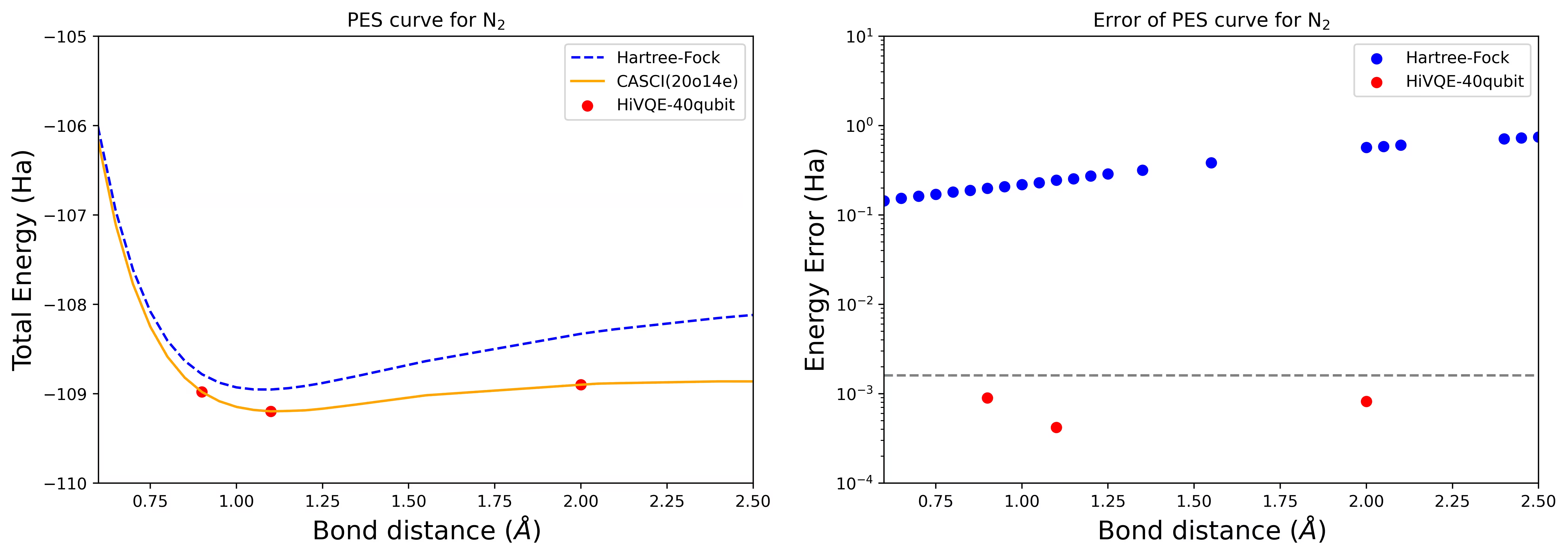
Dissociation PES curve for an N2 molecule with 40 qubits
The nitrogen molecule has been identified as a multireference system with large correlation energy contributions beyond the Hartree-Fock state. We conducted a benchmark calculation for the N2 molecule with cc-pvdz basis, (20o,14e) using the homo-lumo active orbital selection. The complete active space (CAS) number to represent this problem is 6,009,350,400. It is not possible to obtain the eigenvalue problem solution (for energy and electronic structure) with this number of states using a powerful desktop (16cpu/64GB). With HI-VQE, users can efficiently search the subspace of CAS states to find chemically accurate results while saving computation resources significantly. The following plots show the PES curve of 40 qubits HI-VQE calculation of the N2 molecule dissociation.
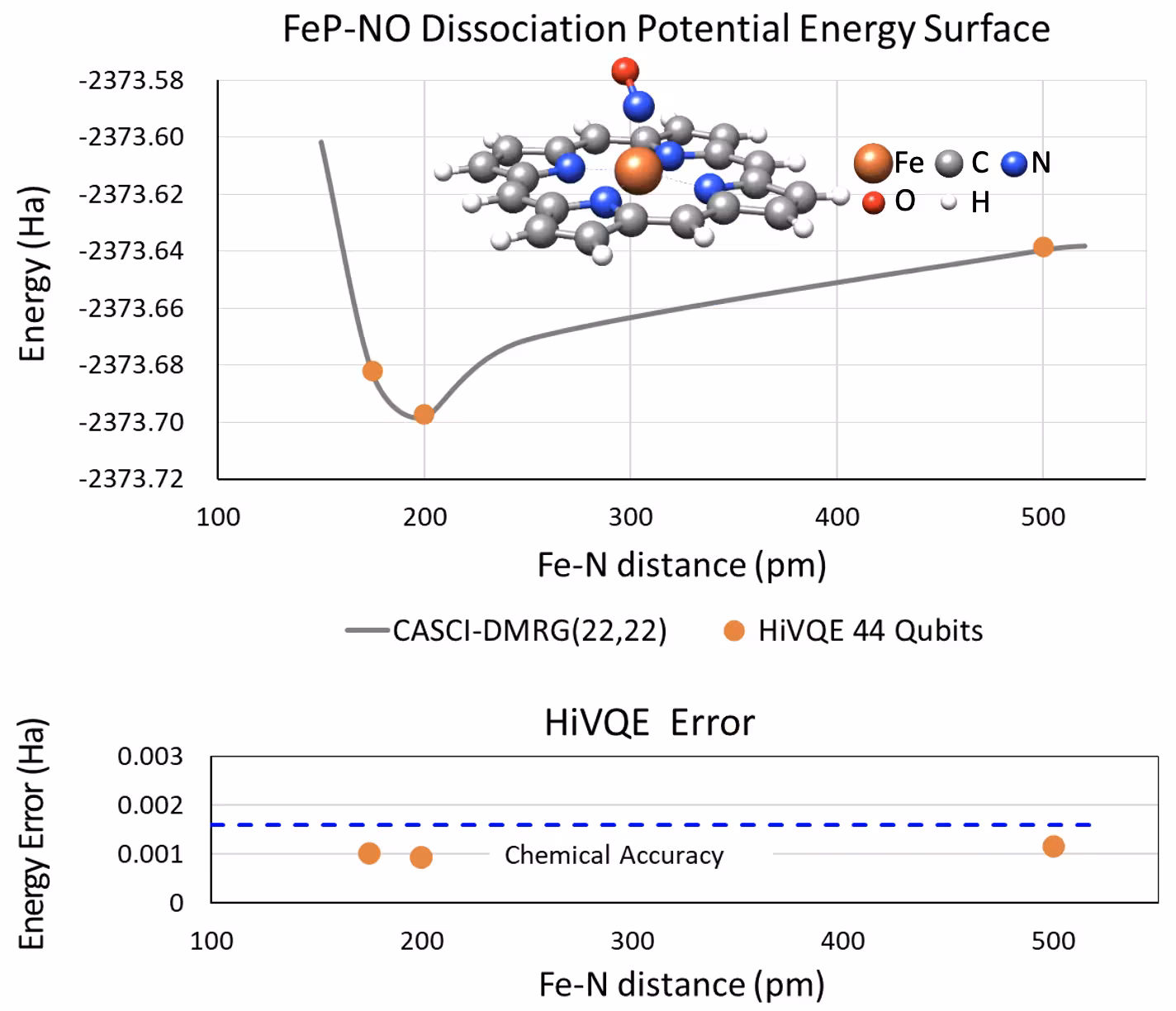
Dissociation PES curve for five-coordinated iron(II)-porphyrin with an NO system with 44 qubits
Another interesting chemical system is an iron(II)-porphyrin (FeP) complex with a coordinated nitric oxide (NO) ligand, which represents a biologically relevant metalloporphyrin system that plays crucial roles in various physiological processes. In this example, HI-VQE has been utilized to estimate the accurate potential energy surface curve of the intermolecular interaction between FeP and NO (ground state energy for differently separated geometries). The combined system has 450 orbitals and 202 electrons (450o,202e) with 6-31g(d) basis in total. The homo-lumo active orbital selection was utilized to calculate the smaller case from the real case with (22o,22e). From the following benchmark results, we were able to achieve the chemical accuracy (> 1.6 mHa) with a state-of-the-art classical computer chemistry calculation of CASCI(DMRG) (22o,22e) reference.
Benchmarks
- Exact matrix size is the number of determinants for exact solution, such as FCI and CASCI.
- HI-VQE calculation samples and calculates the subspace of it (as in, HI-VQE matrix size).
- Total time includes QPU runtime and Qiskit Function runs with CPU.
- Accuracy is estimated from the energy difference from exact solution.
Chemical system | Number of qubits | Exact matrix size | HI-VQE matrix size | E(diff) from exact (mHa) | Number of iteration | Total time | QPU runtime usage |
|---|---|---|---|---|---|---|---|
| (8o,10e) | 16 | 3136 | 1936 | 0.08 | 6 | 37 s | 34 s |
| (10o,10e) | 20 | 63504 | 3969 | 0.60 | 5 | 250 s | 50 s |
| (15o,10e) | 30 | 9018009 | 49729 | 0.90 | 5 | 354 s | 54 s |
| (16o,14e) | 32 | 130873600 | 1798281 | 1.10 | 9 | 6531 s | 121 s |
| (18o,24e) | 36 | 344622096 | 399424 | 0.90 | 24 | 5174 s | 130 s |
| (20o,14e) | 40 | 6009350400 | 9012004 | 1.20 | 21 | 46547 s | 258 s |
Fetch error messages
If your workload fails, the status will be ERROR and calling job.result() will raise an exception:
job = function.run(
    geometry="invalid-geometry",  # This will cause an error
    backend_name=backend_name,
    max_states=2000,
    max_expansion_states=15,
    molecule_options=molecule_options,
    hivqe_options=hivqe_options,
)

job.result()
Output:
---------------------------------------------------------------------------
QiskitServerlessException                 Traceback (most recent call last)
Cell In[12], line 10
      1 job = function.run(
      2     geometry="invalid-geometry",  # This will cause an error
      3     backend_name=backend_name,
   (...)
      7     hivqe_options=hivqe_options,
      8 )
---> 10 job.result()

File ~/work/documentation/documentation/.tox/py311/lib/python3.11/site-packages/qiskit_serverless/core/job.py:253, in Job.result(self, wait, cadence, verbose, maxwait)
    251 if self.status() == "ERROR":
    252     if results:
--> 253         raise QiskitServerlessException(results)
    255     raise QiskitServerlessException(self.filtered_logs(include=r"(?i)error|exception"))
    257 if isinstance(results, str):

QiskitServerlessException: ["runner.UnknownRuntimeError: 'An unexpected error occurred during job execution. Please make sure that your inputs are valid. If you are still experiencing problems, you can contact the Qunova Computing support service at qiskit.support@qunovacomputing.com and provide the Function job ID of this job for more assistance. -- https://docs.quantum.ibm.com/errors#1500'\n"]
job.status()Output:
'ERROR'
Get support
You can send an email to qiskit.support@qunovacomputing.com for help with this function.
If you want help with troubleshooting a specific error, please provide the Function job ID of the job that encountered the error.
Next steps
- Request access to the function by filling in this form.
- Visit the API reference for this Qiskit Function.
- Try the Compute dissociation PES curve for FeP-NO with HI-VQE tutorial.
- Review Pellow-Jarman, A., et al. (2025). HIVQE: Handover Iterative Variational Quantum Eigensolver for Efficient Quantum Chemistry Calculations. arXiv preprint arXiv:2503.06292.
- Try the Dissociation PES curves with Qunova HiVQE tutorial.