QESEM: A Qiskit Function by Qedma
See the API reference
The code on this page was developed using the following requirements. We recommend using these versions or newer.
qiskit[all]~=2.5.0
qiskit-ibm-runtime~=0.47.0
Qiskit Functions are an experimental feature available only to IBM Quantum® Premium Plan, Flex Plan, and On-Prem (via IBM Quantum Platform API) Plan users. They are in preview release status and subject to change.
Overview
While quantum processing units have vastly improved in recent years, errors due to noise and imperfections in existing hardware remain a central challenge for quantum algorithm developers. As the field approaches utility-scale quantum computations that cannot be verified classically, solutions for canceling noise with guaranteed accuracy are becoming increasingly important. To overcome this challenge, Qedma has developed Quantum Error Mitigation (QESEM), seamlessly integrated on IBM Quantum Platform as a Qiskit Function.
With QESEM, users can run their quantum circuits on noisy QPUs to obtain highly accurate error-free results with highly efficient QPU-time overheads, close to fundamental bounds. To achieve this, QESEM leverages a suite of proprietary methods developed by Qedma, for the characterization and reduction of errors. Error reduction techniques include gate optimization, noise-aware transpilation, error suppression (ES), and unbiased error mitigation (EM). With this combination of these characterization-based methods, users can achieve reliable, error-free results for generic large-volume quantum circuits, unlocking applications that cannot be accomplished otherwise.
For a full description of the underlying components, as well as a utility-scale demonstration, refer to the paper Reliable high-accuracy error mitigation for utility-scale quantum circuits.
Description
You can use the QESEM function by Qedma to easily estimate and execute your circuits with error suppression and mitigation, achieving larger circuit volumes and higher accuracies. To use QESEM, you provide a quantum circuit, a set of observables to measure, a target statistical accuracy for each observable, and a chosen QPU. Before you run the circuit to the target accuracy, you can estimate the required QPU time based on an analytical calculation that does not require circuit execution. Once you are satisfied with the QPU time estimation, you can execute the circuit with QESEM.
When you execute a circuit, QESEM runs a device characterization protocol tailored to your circuit, yielding a reliable noise model for the errors occurring in the circuit. Based on the characterization, QESEM first implements noise-aware transpilation to map the input circuit onto a set of physical qubits and gates, which minimizes the noise affecting the target observable. These include the natively available gates (CX/CZ on IBM® devices), as well as additional gates optimized by QESEM, forming QESEM's extended gate set. QESEM then runs a set of characterization-based ES and EM circuits on the QPU and collects their measurement outcomes. These are then classically post-processed to provide an unbiased expectation value and an error bar for each observable, corresponding to the requested accuracy.
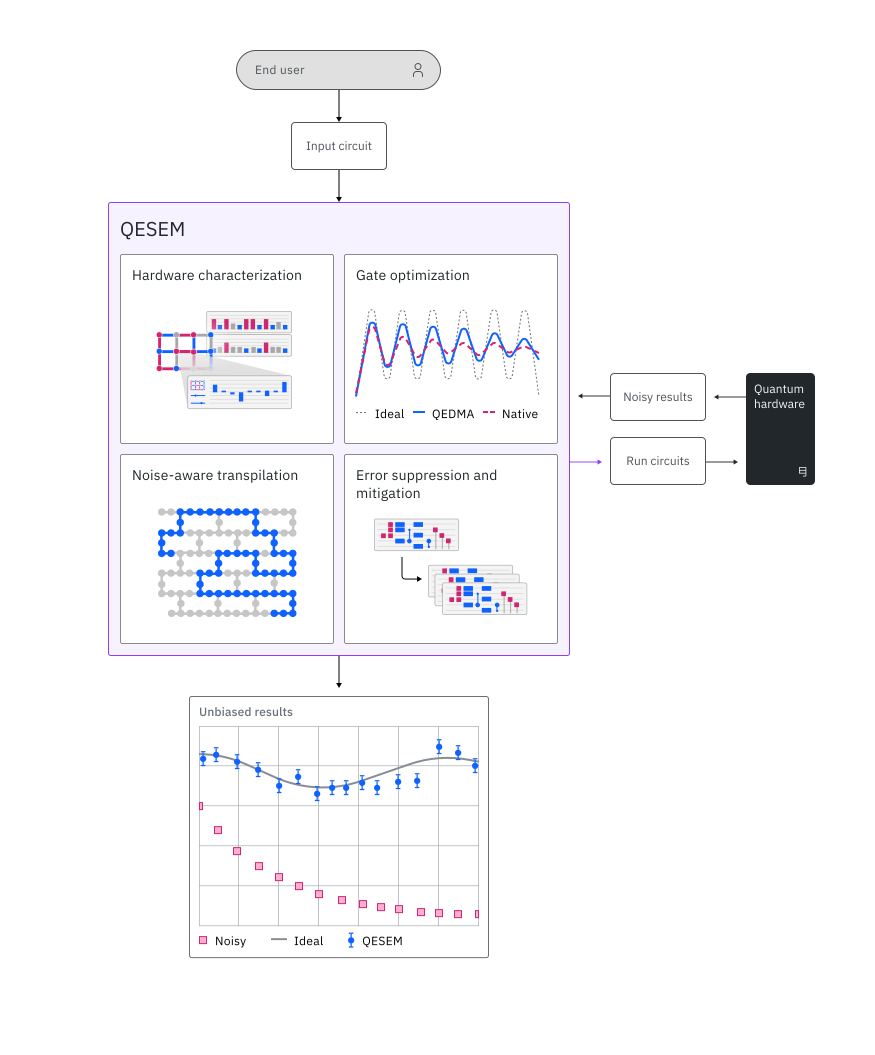
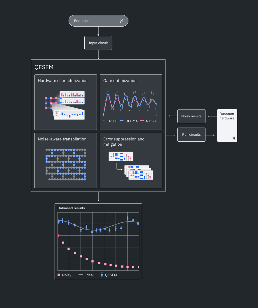
QESEM has been demonstrated to provide high-accuracy results for a variety of quantum applications and on the largest circuit volumes achievable today. QESEM offers the following user-facing features, demonstrated in the benchmarks section below:
- Guaranteed accuracy: QESEM outputs unbiased estimations for expectation values of observables. Its EM method is equipped with theoretical guarantees, which - together with Qedma's cutting-edge characterization - ensure the mitigation converges to the noiseless circuit output up to the user-specified accuracy. In contrast to many heuristic EM methods that are prone to systematic errors or biases, QESEM's guaranteed accuracy is essential for ensuring reliable results in generic quantum circuits and observables.
- Scalability to large QPUs: QESEM's QPU time depends on circuit volumes, but is otherwise independent of the number of qubits. Qedma has demonstrated QESEM on the largest quantum devices available today, including the IBM Quantum 127-qubit Eagle and 133-qubit Heron devices.
- Application-agnostic: QESEM has been demonstrated on a variety of applications, including Hamiltonian simulation, VQE, QAOA, and amplitude estimation. Users can input any quantum circuit and observable to be measured, and obtain accurate error-free results. The only limitations are dictated by the hardware specifications and allocated QPU time, which determine the accessible circuit volumes and output accuracies. In contrast, many error reduction solutions are application-specific or involve uncontrolled heuristics, rendering them inapplicable for generic quantum circuits and applications.
- Extended gate set: QESEM supports fractional-angle gates, and provides Qedma-optimized fractional-angle gates on IBM Quantum Heron and Eagle devices. This extended gate set enables more efficient compilation and unlocks circuit volumes larger by a factor of up to 2 compared to default CX/CZ compilation.
- Multibase observables: QESEM supports input observables composed of many non-commuting Pauli strings, such as generic Hamiltonians. The choice of measurement bases and the optimization of QPU resource allocation (shots and circuits) is then performed automatically by QESEM to minimize the required QPU time for the requested accuracy. This optimization, which takes into account hardware fidelities and execution rates, enables you to run deeper circuits and obtain higher accuracies.
Benchmarks
QESEM has been tested on a wide variety of use cases and applications. The following examples can assist you with assessing which types of workloads you can run with QESEM.
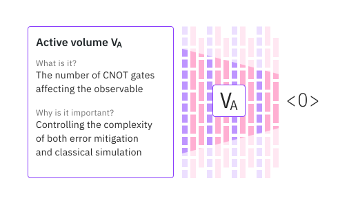
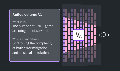
A key figure of merit for quantifying the hardness of both error mitigation and classical simulation for a given circuit and observable is active volume: the number of CNOT gates affecting the observable in the circuit. The active volume depends on the circuit depth and width, on the observable weight, and on the circuit structure, which determines the light cone of the observable. For further details, see the talk from the 2024 IBM Quantum Summit. QESEM provides particularly large value in the high-volume regime, giving reliable results for generic circuits and observables.
Application | Number of qubits | Device | Circuit description | Accuracy | Total time | Runtime usage |
|---|---|---|---|---|---|---|
| VQE circuit | 8 | Eagle (r3) | 21 total layers, 9 measurement bases, 1D chain | 98% | 35 min | 14 min |
| Kicked Ising | 28 | Eagle (r3) | 3 unique layers x 3 steps, 2D heavy-hex topology | 97% | 22 min | 4 min |
| Kicked Ising | 28 | Eagle (r3) | 3 unique layers x 8 steps, 2D heavy-hex topology | 97% | 116 min | 23 min |
| Trotterized Hamiltonian simulation | 40 | Eagle (r3) | 2 unique layers x 10 Trotter steps, 1D chain | 97% | 3 hours | 25 min |
| Trotterized Hamiltonian simulation | 119 | Eagle (r3) | 3 unique layers x 9 Trotter steps, 2D heavy-hex topology | 95% | 6.5 hours | 45 min |
| Kicked Ising | 136 | Heron (r2) | 3 unique layers x 15 steps, 2D heavy-hex topology | 99% | 52 min | 9 min |
Accuracy is measured here relative to the ideal value of the observable: , where '' is the absolute precision of the mitigation (set by the user input), and is the observable at the noiseless circuit. 'Runtime usage' measures the usage of the benchmark in batch mode (sum over usage of individual jobs), whereas 'total time' measures usage in session mode (experiment wall time), which includes additional classical and communication times. QESEM is available for execution in both modes, so that users can make the best use of their available resources.
The 28-qubit Kicked Ising circuits simulate the Discrete Time Quasicrystal studied by Shinjo et al. (see arXiv 2403.16718 and Q2B24 Tokyo) on three connected loops of ibm_kawasaki. The circuit parameters taken here are , with a ferromagnetic initial state . The measured observable is the absolute value of the magnetization . The utility-scale Kicked Ising experiment was run on the 136 best qubits of ibm_fez; this particular benchmark was run at the Clifford angle , at which the active volume grows slowly with circuit depth, which - together with the high device fidelities - enables high accuracy at a short runtime.
Trotterized Hamiltonian simulation circuits are for a Transverse-Field Ising model at fractional angles: and correspondingly (see Q2B24 Tokyo). The utility-scale circuit was run on the 119 best qubits of ibm_brisbane, whereas the 40-qubit experiment was run on the best available chain. The accuracy is reported for the magnetization; high-accuracy results were obtained for higher-weight observables as well.
The VQE circuit was developed together with researchers from the Center for Quantum Technology and Applications at the Deutsches Elektronen-Synchrotron (DESY). The target observable here was a Hamiltonian consisting of a large number of non-commuting Pauli strings, emphasizing QESEM's optimized performance for multi-basis observables. Mitigation was applied to a classically-optimized ansatz; although these results are still unpublished, results of the same quality will be obtained for different circuits with similar structural properties.
Get started
Authenticate using your IBM Quantum Platform API key, and select the QESEM Qiskit Function as follows. (This snippet assumes you've already saved your account to your local environment.)
import qiskit
from qiskit_ibm_catalog import QiskitFunctionsCatalog

catalog = QiskitFunctionsCatalog(channel="ibm_quantum_platform")

# verify that you have access to the function
catalog.list()
# load the function
qesem_function = catalog.load("qedma/qesem")Examples
Time estimation job example
The time estimation job is useful for estimating the QPU time required for a given pub and backend_name. backend_name can also be set to any simulator backend; for example, fake_fez.
QESEM uses a quasi-probabilistic, characterization-based EM method. This method has a QPU time overhead that roughly scales as:
Where is the active volume of the circuit, is the target precision, and is the infidelity of the native gates.
Note that "estimate_time_only": "empirical" uses a few minutes of QPU time to estimate the time required for the job (if the backend is a real device; if it's a simulator, then no QPU time is used). This will usually take around 5 minutes, but no more than 10 minutes. If the infidelity changes drastically between the empirical time estimation job and the mitigation job, the QPU time will also change drastically.
To get started, try this basic example of estimating the required QPU time to run QESEM for a given pub:
backend_name = "fake_fez"

circ = qiskit.QuantumCircuit(5)
circ.cx(0, 1)
circ.cx(2, 3)
circ.cx(1, 2)
circ.cx(3, 4)

avg_magnetization = qiskit.quantum_info.SparsePauliOp.from_sparse_list(
    [("Z", [q], 1 / 5) for q in range(5)], num_qubits=5
)
other_observable = qiskit.quantum_info.SparsePauliOp.from_sparse_list(
    [("ZZ", [0, 1], 1.0), ("XZ", [1, 4], 0.5)], num_qubits=5
)

time_estimation_job = qesem_function.run(
    pubs=[(circ, [avg_magnetization, other_observable])],
    options={
        "estimate_time_only": "empirical",
    },
    backend_name=backend_name,  # example: "fake_fez", "ibm_fez"
)
time_estimate_result = (
time_estimation_job.result()
) # a list of results per pub (circuit)The following code snippet describes how to retrieve different execution metrics from the time estimation job (estimate_time_only is set):
pub_result = time_estimate_result[0]

print(
    f"The estimated QPU time for mitigation for this PUB is: {pub_result.metadata['time_estimation_sec']}"
)
print(
    f"The QPU time that this time estimation job took is (here it is 0 because we used fake_fez): {pub_result.metadata['total_qpu_time']}"
)
print(
    f"Gates fidelity measured during the experiment: {pub_result.metadata['gate_fidelities']}"
)
print(f"Total shots: {pub_result.metadata['total_shots']}")
print(f"Resource usage breakdown: {pub_result.metadata['resource_usage']}")
Output:
The estimated QPU time for mitigation for this PUB is: 300
The QPU time that this time estimation job took is (here it is 0 because we used fake_fez): 0
Gates fidelity measured during the experiment: {'CZ': 0.9951354916722668, 'ID1Q': 0.9991246627329172}
Total shots: 220000
Resource usage breakdown: {'RUNNING: MAPPING': {'CPU_TIME': 33.6066133165732, 'GPU_TIME': 0.0, 'QPU_TIME': 0.0}, 'RUNNING: OPTIMIZING_FOR_HARDWARE': {'CPU_TIME': 184.53575124032795, 'GPU_TIME': 0.0, 'QPU_TIME': 0.0}, 'RUNNING: WAITING_FOR_QPU': {'CPU_TIME': 0.0, 'GPU_TIME': 0.0, 'QPU_TIME': 0.0}, 'RUNNING: EXECUTING_QPU': {'CPU_TIME': 0.0, 'GPU_TIME': 0.0, 'QPU_TIME': 0.0}, 'RUNNING: POST_PROCESSING': {'CPU_TIME': 0.0, 'GPU_TIME': 0.0, 'QPU_TIME': 0.0}}
When empirical time estimation is enabled, QESEM runs a small number of circuits to provide a more accurate QPU time estimate. The mitigation results from these circuits are available in the empirical_estimation_mitigation_results field of the job.
Since these results are derived from a limited sample of circuits, they are significantly less accurate than the final results obtained from the complete QESEM mitigation job. However, when the circuit is small or the target precision is low, the mitigation performed during empirical time estimation may be sufficient to reach the desired precision, and the full mitigation job may not be necessary.
The empirical_estimation_mitigation_results field is a list of PrimitiveResult objects per input parameter. If the circuit is not parametrized, the list will be of length 1.
empirical_estimation_mitigation_results = time_estimate_result[0].metadata[
    "empirical_estimation_mitigation_results"
][0] # a list per parameterprint("Partial results for the observables:")
print(
f" Mitigated expectation values: {empirical_estimation_mitigation_results.data.evs}"
)
print(
f" Mitigated error bars: {empirical_estimation_mitigation_results.data.stds}"
)
print(
f" Number of shots used for mitigation: {empirical_estimation_mitigation_results.metadata['mitigation_shots']}"
)
transpiled_circ = empirical_estimation_mitigation_results.metadata[
"transpiled_circ"
]
print(f" Qubit mapping: {transpiled_circ['qubit_maps']}")
print(
f" Number of measurement bases: {transpiled_circ['num_measurement_bases']}\n"
)
# results per obs
emp_obs_results = empirical_estimation_mitigation_results.metadata["results"][
0
]
# print(f"Results for each observable: {results}")
print("Results for each observable:")
for i, (obs_array, result_dict) in enumerate(emp_obs_results):
# obs_array, result_dict = results
print(f"Observable {i+1}: {obs_array}")
print(
f" QESEM mitigated value: {result_dict['qesem']['value']} \u00b1 {result_dict['qesem']['error_bar']}"
)Output:
Partial results for the observables:
    Mitigated expectation values: [1.00347302 1.00693905]
    Mitigated error bars: [0.00304061 0.00714276]
    Number of shots used for mitigation: 180000
    Qubit mapping: [[[0, 136], [1, 143], [2, 142], [3, 141], [4, 140]]]
    Number of measurement bases: 2

Results for each observable:
Observable 1: ObservablesArray({'IIIIZ': 0.2, 'IIIZI': 0.2, 'IIZII': 0.2, 'IZIII': 0.2, 'ZIIII': 0.2}, shape=())
    QESEM mitigated value: 1.003473015776871 ± 0.0030406128032204015
Observable 2: ObservablesArray({'IIIZZ': 1.0, 'ZIIXI': 0.5}, shape=())
    QESEM mitigated value: 1.0069390542613554 ± 0.0071427606736885925
QESEM mitigation job example
The following example executes a QESEM job:
sample_job = qesem_function.run(
    pubs=[(circ, [avg_magnetization, other_observable])],
    backend_name=backend_name,  # example: "ibm_fez"
    # options = {
    #     "estimate_time_only": "empirical",
    #     "default_precision": 0.2,  # Default precision is applied to all pubs that don't have a precision specified, see API reference for more details
    #     "max_execution_time": 3600,  # You can specify a maximum QPU time in seconds, see API reference for more details
    #     "transpilation_level": "standard",  # "minimal_with_layout_opt" for minimal transpilation, see API reference for more details
    #     "parallel_execution": True,  # True for parallel execution, see API reference for more details
    # },
)
For a detailed description of each input field and option, see the QESEM API reference.
You can use the familiar Qiskit Serverless APIs to check your Qiskit Function workload's status or return results:
# Print the ID so you can use it later, if necessary
print(sample_job.job_id)
print(sample_job.status())
sample_result = sample_job.result()
Output:
3ac6b2df-15b0-4dc0-8f48-cf14bd20a1c8
DONE
The following code snippet demonstrates how to retrieve the mitigation results and execution metrics. These contain essential data that enables a deeper understanding of how different parameters impact the QESEM execution. It may also be relevant when writing a paper based on your research.
for pub_idx, pub_result in enumerate(
    sample_result
):  # each element in the list is a result for a different pub, here we sent only one pub
    print(f"\nPUB {pub_idx}:")
    print(
        f"  The QPU time that this job took is (here it is 0 because we used fake_fez): {pub_result.metadata['total_qpu_time']}"
    )
    print(
        f"  Gates fidelity measured during the experiment: {pub_result.metadata['gate_fidelities']}"
    )
    print(f"  Total shots: {pub_result.metadata['total_shots']}")
    print(
        f"  Number of shots used for mitigation: {pub_result.metadata['mitigation_shots']}"
    )
    print(
        f"  Resource usage breakdown: {pub_result.metadata['resource_usage']}"
    )
Output:
PUB 0:
  The QPU time that this job took is (here it is 0 because we used fake_fez): 0.0
  Gates fidelity measured during the experiment: {'CZ': 0.9953704216147041, 'ID1Q': 0.9991834123567518}
  Total shots: 446000
  Number of shots used for mitigation: 194000
  Resource usage breakdown: {'RUNNING: MAPPING': {'CPU_TIME': 32.52745003718883, 'GPU_TIME': 0.0, 'QPU_TIME': 0.0}, 'RUNNING: OPTIMIZING_FOR_HARDWARE': {'CPU_TIME': 257.850521848537, 'GPU_TIME': 0.0, 'QPU_TIME': 0.0}, 'RUNNING: WAITING_FOR_QPU': {'CPU_TIME': 0.0, 'GPU_TIME': 0.0, 'QPU_TIME': 0.0}, 'RUNNING: EXECUTING_QPU': {'CPU_TIME': 0.0, 'GPU_TIME': 0.0, 'QPU_TIME': 0.0}, 'RUNNING: POST_PROCESSING': {'CPU_TIME': 0.0, 'GPU_TIME': 0.0, 'QPU_TIME': 0.0}}
In metadata["results"], results are grouped first by circuit instance and then by observable.
print("Full QESEM mitigation results:")

for pub_idx, pub_result in enumerate(sample_result):
    print(f"\nPUB {pub_idx}:")

    print(f"  Mitigated expectation values: {pub_result.data.evs}")
    print(f"  Mitigated error bars: {pub_result.data.stds}")
    noisy_results = pub_result.metadata.get("noisy_results")
    print(f"  Unmitigated expectation values: {noisy_results.evs}")
    print(f"  Unmitigated error bars: {noisy_results.stds}")

    print("  Transpiled circuits:")
    for circ_idx, transpiled_circ in enumerate(
        pub_result.metadata["transpiled_circs"]
    ):
        print(f"    Circuit {circ_idx}:")
        # print(f"      Circuit: \n {transpiled_circ['circuit']}") # not printing it because it's long but you can see the transpiled circuit itself
        print(f"      Qubit mapping: {transpiled_circ['qubit_maps']}")
        print(
            f"      Measurement bases: {transpiled_circ['num_measurement_bases']}"
        )

    print("  Results for each observable:")
    for circ_idx, circ_results in enumerate(pub_result.metadata["results"]):
        print(f"    Circuit {circ_idx}:")
        for obs_idx, (obs_array, result_dict) in enumerate(circ_results):
            print(f"      Observable {obs_idx}: {obs_array}")
            print(
                f"        QESEM mitigated value: {result_dict['qesem']['value']} ± {result_dict['qesem']['error_bar']}"
            )
            print(
                f"        Unmitigated value: {result_dict['unmitigated']['value']} ± {result_dict['unmitigated']['error_bar']}"
            )
Output:
Full QESEM mitigation results:

PUB 0:
  Mitigated expectation values: [1.00648343 1.00636289]
  Mitigated error bars: [0.00253812 0.00693586]
  Unmitigated expectation values: [0.98031429 0.96357143]
  Unmitigated error bars: [0.00124128 0.00578812]
  Transpiled circuits:
    Circuit 0:
      Qubit mapping: [[[0, 140], [1, 141], [2, 142], [3, 143], [4, 136]]]
      Measurement bases: 2
  Results for each observable:
    Circuit 0:
      Observable 0: ObservablesArray({'IIIIZ': 0.2, 'IIIZI': 0.2, 'IIZII': 0.2, 'IZIII': 0.2, 'ZIIII': 0.2}, shape=())
        QESEM mitigated value: 1.0064834305181962 ± 0.002538119914534849
        Unmitigated value: 0.9803142857142859 ± 0.0012412835813609938
      Observable 1: ObservablesArray({'IIIZZ': 1.0, 'ZIIXI': 0.5}, shape=())
        QESEM mitigated value: 1.0063628870614818 ± 0.006935859820870656
        Unmitigated value: 0.9635714285714285 ± 0.005788121870526659
Main results breakdown:
mitigated: the fully mitigated QESEM expectation value.unmitigated: the raw physical-noise result without error mitigation.
QESEM heuristic extrapolation results
In a standard QESEM run with a single precision float, the results also include automatically available noise-scaling points that are used for the QESEM heuristic. These points are computed without additional QPU resources.
Scale 1.0 represents the physical device noise level with readout mitigation (REM), while scale 2.0 is the complementary noise-amplified point, also with REM. These points are used to produce the qesem_heuristic result.
qesem_heuristic: a ZNE-style estimate computed from the available noise-scaled data. Currently, this uses exponential extrapolation.noise_scaling.results_with_REM: expectation values at different noise scales, all with readout mitigation (REM).
A subtle but important detail is that the scale 1.0 result is not the same as the unmitigated result. Both correspond to the physical device noise level, but the scale 1.0 point includes readout mitigation, while unmitigated does not.
print("QESEM heuristic results:")

for pub_idx, pub_result in enumerate(sample_result):
    print(f"\nPUB {pub_idx}:")
    for circ_idx, circ_results in enumerate(pub_result.metadata["results"]):
        print(f"  Circuit {circ_idx}:")
        for obs_idx, (obs_array, result_dict) in enumerate(circ_results):
            print(f"    Observable {obs_idx}: {obs_array}")
            qesem_heuristic = result_dict["qesem_heuristic"][0]
            print("      QESEM heuristic:")
            print(
                f"        Value: {qesem_heuristic['value']} ± {qesem_heuristic['error_bar']}"
            )
            print(
                f"        Extrapolation: {qesem_heuristic['extrapolation']}"
            )
            print(
                f"        Scale factors: {qesem_heuristic['scale_factors']}"
            )
            noise_scaling = result_dict["noise_scaling"]
            print("      Noise scaling results:")
            print(
                f"        Scaling method: {noise_scaling['scaling_method']}"
            )
            print("        Results with Readout mitigation (REM):")
            for rem_result in sorted(
                (
                    item
                    for item in noise_scaling["results_with_REM"]
                    if item["scale"] != 0.0
                ),
                key=lambda item: item["scale"],
            ):
                print(
                    f"          Scale factor {rem_result['scale']}: {rem_result['value']} ± {rem_result['error_bar']}"
                )
Output:
QESEM heuristic results:

PUB 0:
  Circuit 0:
    Observable 0: ObservablesArray({'IIIIZ': 0.2, 'IIIZI': 0.2, 'IIZII': 0.2, 'IZIII': 0.2, 'ZIIII': 0.2}, shape=())
      QESEM heuristic:
        Value: 1.0008161638888535 ± 0.0038859458884403964
        Extrapolation: exponential
        Scale factors: [1.0, 2.0]
      Noise scaling results:
        Scaling method: QESEM
        Results with Readout mitigation (REM):
          Scale factor 1.0: 0.9918395459270772 ± 0.0012565417579355634
          Scale factor 2.0: 0.982943441922748 ± 0.0028919278067695018
    Observable 1: ObservablesArray({'IIIZZ': 1.0, 'ZIIXI': 0.5}, shape=())
      QESEM heuristic:
        Value: 0.9960853148925298 ± 0.013811635038961175
        Extrapolation: exponential
        Scale factors: [1.0, 2.0]
      Noise scaling results:
        Scaling method: QESEM
        Results with Readout mitigation (REM):
          Scale factor 1.0: 0.9902860583785115 ± 0.005921236914723409
          Scale factor 2.0: 0.984520565414274 ± 0.006909522262347639
The following examples focus on feature-specific inputs and results, so they do not print the full execution metrics each time. The top-level metadata shown earlier, such as total_qpu_time, gate_fidelities, total_shots, mitigation_shots, and resource_usage, is available for these jobs as well.
Some variables from the previous examples, including the backend, observables, and base circuit parameters, are reused below for conciseness.
All of the following examples can also be run with empirical time estimation. To enable it, pass "estimate_time_only": "empirical" in the function options.
Parameterized circuit example
Many algorithms evaluate the same circuit at several parameter values. Sending the parameterized circuit as one QESEM job lets QESEM share characterization and calibration across the circuit instances, which can reduce QPU-time overhead compared with running separate jobs.
Submitting a parameterized circuit requires using the "minimal_with_layout_opt" transpilation level.
Circuits submitted at this level should already be expressed using the backend's basis gates, depending on the backend. At this level, QESEM keeps the submitted structure as close as possible to the input circuit, respects barriers during layerification (grouping operations into layers of parallel two-qubit gates), and still handles hardware mapping to high-fidelity qubits and device connectivity automatically.
In practice, this means you should transpile circuits to the target backend’s basis gates before submission. A simple basis-gate transpilation example is shown below.
QESEM currently supports only one observable per parameter set. The two parameter rows below are zipped with the two observables: the first row is measured with avg_magnetization, and the second row is measured with other_observable.
# Transpile to the backend basis gates only. With minimal_with_layout_opt, QESEM handles hardware mapping/connectivity and observable layout internally.
from qiskit_ibm_runtime.fake_provider import FakeFez

backend = FakeFez()
basis = backend.operation_names
print(basis)

param0 = qiskit.circuit.Parameter("param0")
param1 = qiskit.circuit.Parameter("param1")
parametrized_circ = qiskit.QuantumCircuit(5)
parametrized_circ.rx(param0, 0)
parametrized_circ.rx(param1, 1)
parametrized_circ.cx(0, 1)
parametrized_circ.cx(2, 3)
parametrized_circ.cx(1, 2)
parametrized_circ.cx(3, 4)

parametrized_circ = qiskit.transpile(
    parametrized_circ, basis_gates=basis, optimization_level=1
)
parametrized_parameter_values = [[0.5, 0.1], [0.0, 0.6]]
parametrized_observables = [avg_magnetization, other_observable]

parametrized_job = qesem_function.run(
    pubs=[
        (
            parametrized_circ,
            parametrized_observables,
            parametrized_parameter_values,
            0.1,
        )
    ],
    backend_name=backend_name,
    options={
        "max_execution_time": 300,
        "transpilation_level": "minimal_with_layout_opt",
    },
)print(parametrized_job.job_id)
print(parametrized_job.status())Output:
d1b0e29b-196c-4896-aec6-44a268ebd874
DONE
parametrized_result = parametrized_job.result()print("Parameterized circuit QESEM results:")
for pub_idx, pub_result in enumerate(parametrized_result):
print(f"\nPUB {pub_idx}:")
print(f" Mitigated expectation values: {pub_result.data.evs}")
print(f" Mitigated error bars: {pub_result.data.stds}")
noisy_results = pub_result.metadata["noisy_results"]
print(f" Unmitigated expectation values: {noisy_results.evs}")
print(f" Unmitigated error bars: {noisy_results.stds}")
print(" Results for each parameter value:")
for param_idx, param_results in enumerate(pub_result.metadata["results"]):
print(
f" Parameter set {param_idx}: {parametrized_parameter_values[param_idx]}"
)
for obs_idx, (obs_array, result_dict) in enumerate(param_results):
print(f" Observable {obs_idx}: {obs_array}")
print(
f" QESEM mitigated value: {result_dict['qesem']['value']} ± {result_dict['qesem']['error_bar']}"
)
print(
f" Unmitigated value: {result_dict['unmitigated']['value']} ± {result_dict['unmitigated']['error_bar']}"
)Output:
Parameterized circuit QESEM results:

PUB 0:
  Mitigated expectation values: [0.92392021 0.82517653]
  Mitigated error bars: [0.00565281 0.00616016]
  Unmitigated expectation values: [0.9028     0.78771429]
  Unmitigated error bars: [0.00335142 0.00925413]
  Results for each parameter value:
    Parameter set 0: [0.5, 0.1]
      Observable 0: ObservablesArray({'IIIIZ': 0.2, 'IIIZI': 0.2, 'IIZII': 0.2, 'IZIII': 0.2, 'ZIIII': 0.2}, shape=())
        QESEM mitigated value: 0.923920210615709 ± 0.005652811570890183
        Unmitigated value: 0.9028 ± 0.0033514176105045447
    Parameter set 1: [0.0, 0.6]
      Observable 0: ObservablesArray({'IIIZZ': 1.0, 'ZIIXI': 0.5}, shape=())
        QESEM mitigated value: 0.8251765289285893 ± 0.006160161743353999
        Unmitigated value: 0.7877142857142858 ± 0.009254130564027902
Multi-pub example
Multi-pub execution is useful when you want to run several related circuits in one QESEM job. Like parameterized execution, this can reduce overhead because QESEM can share characterization and calibration across circuit instances instead of repeating it in separate jobs.
This is especially useful for circuits with a shared layer structure, such as Trotter-type workloads, where different circuits reuse the same unique layers. In that case, running them together can reduce characterization cost compared with independent QESEM jobs.
Multi-pub jobs require "transpilation_level": "minimal_with_layout_opt". As in the parameterized example, the circuits should be transpiled to the target backend’s basis gates before submission. QESEM then handles device connectivity, layout, and mapping to high-fidelity qubits internally.
Each PUB below contains one circuit and the same two observables used earlier in the notebook, so the returned PrimitiveResult contains one PubResult per input circuit.
The example below uses two simple Trotter circuits with the same layer pattern: circ_a has one Trotter layer, and circ_b repeats the same layer pattern twice. This makes the shared structure explicit.
def make_trotter_circuit(num_qubits, num_layers, zz_angle=0.2, x_angle=0.1):
    trotter_circ = qiskit.QuantumCircuit(num_qubits)
    for _ in range(num_layers):
        for q in range(num_qubits):
            trotter_circ.rx(x_angle, q)
        trotter_circ.barrier()
        for q in range(0, num_qubits - 1, 2):
            trotter_circ.rzz(zz_angle, q, q + 1)
        trotter_circ.barrier()
        for q in range(1, num_qubits - 1, 2):
            trotter_circ.rzz(zz_angle, q, q + 1)
        trotter_circ.barrier()
    return trotter_circ


circ_a = make_trotter_circuit(num_qubits=5, num_layers=1)
circ_b = make_trotter_circuit(num_qubits=5, num_layers=2)
multi_pubs = [
(
qiskit.transpile(qci, basis_gates=basis, optimization_level=1),
[avg_magnetization, other_observable],
)
for qci in [circ_a, circ_b]
]
multi_circ_job = qesem_function.run(
pubs=multi_pubs,
backend_name=backend_name,
options={
"max_execution_time": 300,
"transpilation_level": "minimal_with_layout_opt",
"default_precision": 0.1,
},
)print(multi_circ_job.job_id)
print(multi_circ_job.status())Output:
e34565b8-7262-4133-a120-de42ce624a99
DONE
multi_circ_result = multi_circ_job.result()print("Multi-pub QESEM results:")
for pub_idx, pub_result in enumerate(multi_circ_result):
print(f"\nPUB {pub_idx}:")
print(f" Mitigated expectation values: {pub_result.data.evs}")
print(f" Mitigated error bars: {pub_result.data.stds}")
noisy_results = pub_result.metadata["noisy_results"]
print(f" Unmitigated expectation values: {noisy_results.evs}")
print(f" Unmitigated error bars: {noisy_results.stds}")
print(" Results for each observable:")
for circ_idx, circ_results in enumerate(pub_result.metadata["results"]):
print(f" Circuit {circ_idx}:")
for obs_idx, (obs_array, result_dict) in enumerate(circ_results):
print(f" Observable {obs_idx}: {obs_array}")
print(
f" QESEM mitigated value: {result_dict['qesem']['value']} ± {result_dict['qesem']['error_bar']}"
)
print(
f" Unmitigated value: {result_dict['unmitigated']['value']} ± {result_dict['unmitigated']['error_bar']}"
)Output:
Multi-pub QESEM results:

PUB 0:
  Mitigated expectation values: [0.99502406 1.02209332]
  Mitigated error bars: [0.00483819 0.00707488]
  Unmitigated expectation values: [0.96934286 0.97271429]
  Unmitigated error bars: [0.00124855 0.00617294]
  Results for each observable:
    Circuit 0:
      Observable 0: ObservablesArray({'IIIIZ': 0.2, 'IIIZI': 0.2, 'IIZII': 0.2, 'IZIII': 0.2, 'ZIIII': 0.2}, shape=())
        QESEM mitigated value: 0.9950240647925642 ± 0.004838188086259301
        Unmitigated value: 0.9693428571428573 ± 0.0012485470362492692
      Observable 1: ObservablesArray({'IIIZZ': 1.0, 'ZIIXI': 0.5}, shape=())
        QESEM mitigated value: 1.0220933230604674 ± 0.007074884384355636
        Unmitigated value: 0.9727142857142859 ± 0.006172939375512439

PUB 1:
  Mitigated expectation values: [0.98850017 1.02555188]
  Mitigated error bars: [0.0077912  0.01672652]
  Unmitigated expectation values: [0.93682857 0.95371429]
  Unmitigated error bars: [0.00156245 0.00665735]
  Results for each observable:
    Circuit 0:
      Observable 0: ObservablesArray({'IIIIZ': 0.2, 'IIIZI': 0.2, 'IIZII': 0.2, 'IZIII': 0.2, 'ZIIII': 0.2}, shape=())
        QESEM mitigated value: 0.988500171577252 ± 0.007791203181151346
        Unmitigated value: 0.9368285714285716 ± 0.001562451883089579
      Observable 1: ObservablesArray({'IIIZZ': 1.0, 'ZIIXI': 0.5}, shape=())
        QESEM mitigated value: 1.02555188098689 ± 0.016726524388086233
        Unmitigated value: 0.9537142857142858 ± 0.006657345655544263
Quasi-probabilistic Error Tuning (QET) example
Quasi-probabilistic Error Tuning (QET) requests expectation values at selected noise scale factors. This is useful for custom noise-scaling studies and Zero-Noise Extrapolation workflows. Scale 1.0 is the physical noise level, values between 0.0 and 1.0 partially reduce noise, and values above 1.0 amplify noise.
To use QET with the Qiskit Function, pass a dictionary as the PUB precision. The dictionary maps each requested noise scale to its target precision. Returned scale-factor results are stored in noise_scaling.results_with_REM and include readout mitigation. The scale 1.0 point is therefore not identical to the unmitigated value, because 1.0 includes readout mitigation while unmitigated does not.
When a scale is requested, QESEM also returns the complementary scale around 1.0 without extra QPU usage. For example, requesting 0.5 can also return 1.5, and requesting 1.3 can also return 0.7. The precision on the complementary scale is not guaranteed.
noise_scale_precision = {0.5: 0.15, 1.3: 0.2}

qet_job = qesem_function.run(
    pubs=[
        (
            circ,
            [avg_magnetization, other_observable],
            None,
            noise_scale_precision,
        )
    ],
    backend_name=backend_name,
    options={"max_execution_time": 300},
)print(qet_job.job_id)
print(qet_job.status())Output:
8195fa58-f037-4651-8715-36ce1cdc5521
DONE
qet_result = qet_job.result()print("QET noise-scaling results:")
for pub_idx, pub_result in enumerate(qet_result):
print(f"\nPUB {pub_idx}:")
noisy_results = pub_result.metadata["noisy_results"]
print(f" Unmitigated expectation values: {noisy_results.evs}")
print(f" Unmitigated error bars: {noisy_results.stds}")
print(" Results for each observable:")
for circ_idx, circ_results in enumerate(pub_result.metadata["results"]):
print(f" Circuit {circ_idx}:")
for obs_idx, (obs_array, result_dict) in enumerate(circ_results):
print(f" Observable {obs_idx}: {obs_array}")
noise_scaling = result_dict["noise_scaling"]
print(
f" Scaling method: {noise_scaling['scaling_method']}"
)
print(" Results with Readout mitigation (REM):")
for rem_result in sorted(
(
item
for item in noise_scaling["results_with_REM"]
if item["scale"] != 0.0
),
key=lambda item: item["scale"],
):
print(
f" Scale factor {rem_result['scale']}: {rem_result['value']} ± {rem_result['error_bar']}"
)Output:
QET noise-scaling results:

PUB 0:
  Unmitigated expectation values: [0.97822857 0.96171429]
  Unmitigated error bars: [0.00123812 0.00672958]
  Results for each observable:
    Circuit 0:
      Observable 0: ObservablesArray({'IIIIZ': 0.2, 'IIIZI': 0.2, 'IIZII': 0.2, 'IZIII': 0.2, 'ZIIII': 0.2}, shape=())
        Scaling method: QESEM
        Results with Readout mitigation (REM):
          Scale factor 0.5: 0.9938730340199383 ± 0.0032116907357568275
          Scale factor 0.7: 0.9963976191853445 ± 0.00036300258869586616
          Scale factor 1.0: 0.9898115079506586 ± 0.0012525947426560995
          Scale factor 1.3: 0.9864667065580341 ± 0.002633221613518526
          Scale factor 1.5: 0.9838755527197551 ± 0.002948417797996015
      Observable 1: ObservablesArray({'IIIZZ': 1.0, 'ZIIXI': 0.5}, shape=())
        Scaling method: QESEM
        Results with Readout mitigation (REM):
          Scale factor 0.5: 1.0006538544450332 ± 0.002121742014777343
          Scale factor 0.7: 1.0004159801523036 ± 0.0021671375357823794
          Scale factor 1.0: 0.9898058846339917 ± 0.00690183710903159
          Scale factor 1.3: 0.9948946719997267 ± 0.002146532859610311
          Scale factor 1.5: 0.9927220368192772 ± 0.0020875057190323882
Fetch error messages
If your workload status is ERROR, use job.result() to fetch the error message as follows:
# Get the result and truncate for readability
result = sample_job.result()
result_str = str(result)
max_length = 500  # Adjust this value as necessary

if len(result_str) > max_length:
    truncated = (
        result_str[:max_length]
        + f"... (truncated {len(result_str) - max_length} characters)"
    )
else:
    truncated = result_str

print(truncated)
Output:
PrimitiveResult([PubResult(data=DataBin(evs=np.ndarray(<shape=(2,), dtype=float64>), stds=np.ndarray(<shape=(2,), dtype=float64>), shape=(2,)), metadata={'gate_fidelities': {'CZ': 0.9979444718552628, 'ID1Q': 0.9991994239814883}, 'total_shots': 498600, 'mitigation_shots': 223400, 'transpiled_circs': [{'circuit': 'OPENQASM 3.0;\ninclude "stdgates.inc";\nbit[76] c0;\nqubit[76] q0;\nrx(0) q0[54];\nrx(0) q0[59];\nrx(0) q0[75];\nrz(pi/2) q0[54];\nrz(pi/2) q0[59];\nrz(pi/2) q0[75];\nrx(pi/2) q0[54];\nr... (truncated 3771 characters)
Get support
The Qedma support team is here to help! If you encounter any issues or have questions about using the QESEM Qiskit Function, please don't hesitate to reach out. Our knowledgeable and friendly support staff are ready to assist you with any technical concerns or inquiries you may have.
You can email us at support@qedma.com for assistance. Please include as much detail as possible about the issue you're experiencing to help us provide a swift and accurate response. You can also contact your dedicated Qedma POC representative via email or phone.
To help us assist you more efficiently, please provide the following information when you contact us:
- A detailed description of the issue
- The job ID
- Any relevant error messages or codes
We are committed to providing you with prompt and effective support to ensure you have the best possible experience with our Qiskit Function.
We are always looking to improve our product and we welcome your suggestions! If you have ideas on how we can enhance our services or features you'd like to see, please send us your thoughts at support@qedma.com.
Next steps
- Request access to Qedma QESEM.
- Visit the API reference for this Qiskit Function.
- Try the Simulate 2D tilted-field Ising with the QESEM function tutorial.
- Review Aharonov, D., et al. (2025). Reliable high-accuracy error mitigation for utility-scale quantum circuits. arXiv preprint arXiv:2508.10997.
- Review Aharonov, D., et al. (2025). Syndrome aware mitigation of logical errors. arXiv preprint arXiv:2508.10997.
- Review Aharonov, D., et al. (2025). On the Importance of Error Mitigation for Quantum Computation. arXiv preprint arXiv:2512.23810.
- Review Bauman, N. P., et al. (2025). Coupled Cluster Downfolding Theory in Simulations of Chemical Systems on Quantum Hardware. arXiv preprint arXiv:2507.01199.
- Review Goldack, M., et al. (2026). Computing Statistical Properties of Velocity Fields on Current Quantum Hardware. arXiv preprint arXiv:2601.10166.
- Review Sakuma, R., et al. (2026). Point-group symmetry analysis of many-electron wavefunctions on a quantum computer arXiv preprint arXiv:2605.24824.