Performance Management: A Qiskit Function by Q-CTRL Fire Opal

Note

Qiskit Functions are an experimental feature available only to IBM Quantum® Premium Plan, Flex Plan, and On-Prem (via IBM Quantum Platform API) Plan users. They are in preview release status and subject to change.

The code on this page was developed using the following requirements. We recommend using these versions or newer.
```
qiskit[all]~=2.3.1
qiskit-ibm-runtime~=0.45.1
```

Overview

Fire Opal Performance Management makes it simple for anyone to achieve meaningful results from quantum computers at scale without needing to be quantum hardware experts. When running circuits with Fire Opal Performance Management, AI-driven error suppression techniques are automatically applied, enabling the scaling of larger problems with more gates and qubits. This approach reduces the number of shots required to reach the correct answer, with no added overhead — resulting in significant savings in both compute time and cost.

Performance Management suppresses errors and increases the probability of getting the correct answer on noisy hardware. In other words, it increases the signal-to-noise ratio. The following image shows how increased accuracy enabled by Performance Management can reduce the need for additional shots in the case of a 10-qubit Quantum Fourier Transform algorithm. With only 30 shots, Q-CTRL reaches the 99% confidence threshold, whereas the default (QiskitRuntime Sampler, optimization_level=3 and resilience_level=1, ibm_sherbrooke) requires 170,000 shots. By getting the right answer faster, you save significant compute runtime.

The Performance Management function can be used with any algorithm, and you can easily use it in place of the standard Qiskit Runtime primitives. Behind the scenes, multiple error suppression techniques work together to prevent errors from happening at runtime. All Fire Opal pipeline methods are pre-configured and algorithm-agnostic, meaning you always get the best performance out of the box.

To get access to Performance Management, contact Q-CTRL.

Description

Fire Opal Performance Management has two options for execution that are similar to the Qiskit Runtime primitives, so you can easily swap in the Q-CTRL Sampler and Estimator. The general workflow for using the Performance Management function is:

Define your circuit (and operators in the case of the Estimator).
Run the circuit.
Retrieve the results.

To reduce hardware noise, Fire Opal employs a range of AI-driven error suppression techniques depicted in the following image. With Fire Opal, the entire pipeline is completely automated with zero need for configuration.

Fire Opal's pipeline eliminates the need for additional overhead, such as increased quantum runtime or extra physical qubits. Note that classical processing time remains a factor (refer to the Benchmarks section for estimates, where "Total time" reflects both classical and quantum processing). In contrast to error mitigation, which requires overhead in the form of sampling, Fire Opal's error suppression works at both the gate and pulse levels to address various sources of noise and to prevent the likelihood of an error occurring. By preventing errors, the need for expensive post-processing is eliminated.

The following image depicts the error suppression methods automated by Fire Opal Performance Management.

Visualization of the error suppression pipeline

The function offers two primitives, Sampler and Estimator, and the inputs and outputs of both extend the implemented spec for Qiskit Runtime V2 primitives.

Benchmarks

Published algorithmic benchmarking results demonstrate significant performance improvement across various algorithms, including Bernstein-Vazirani, quantum Fourier transform, Grover’s search, quantum approximate optimization algorithm, and variational quantum eigensolver. The rest of this section provides more details about types of algorithms you can run, as well as the expected performance and runtimes.

The following independent studies demonstrate how Q-CTRL's Performance Management enables algorithmic research at record-breaking scale:

Parametrized Energy-Efficient Quantum Kernels for Network Service Fault Diagnosis - up to 50-qubit quantum kernel learning
Tensor-based quantum phase difference estimation for large-scale demonstration - up to 33-qubit quantum phase estimation
Hierarchical Learning for Quantum ML: Novel Training Technique for Large-Scale Variational Quantum Circuits - up to 21-qubit quantum data loading

The following table provides a rough guide on accuracy and runtimes from prior benchmarking runs on ibm_fez. Performance on other devices may vary. The usage time is based on an assumption of 10,000 shots per circuit. The "Number of qubits" indicated is not a hard limitation but represents rough thresholds where you can expect extremely consistent solution accuracy. Larger problem sizes have been successfully solved, and testing beyond these limits is encouraged.

Example	Number of qubits	Accuracy	Measure of accuracy	Total time (s)	Runtime usage (s)	Primitive (Mode)
Bernstein–Vazirani	50Q	100%	Success Rate (Percentage of runs where the correct answer is the highest count bitstring)	10	8	Sampler
Quantum Fourier Transform	30Q	100%	Success Rate (Percentage of runs where the correct answer is the highest count bitstring)	10	8	Sampler
Quantum Phase Estimation	30Q	99.9998%	Accuracy of the angle found: `1- abs(real_angle - angle_found)/pi`	10	8	Sampler
Quantum simulation: Ising model (15 steps)	20Q	99.775%	$A$ (defined below)	60 (per step)	15 (per step)	Estimator
Quantum simulation 2: molecular dynamics (20 time points)	34Q	96.78%	$A_{mean}$ (defined below)	10 (per time point)	6 (per time point)	Estimator

Defining the accuracy of the measurement of an expectation value - the metric $A$ is defined as follows:

A = 1 - \frac{|\epsilon^{ideal} - \epsilon^{meas}|}{\epsilon^{ideal}_{max} - \epsilon^{ideal}_{min}},

where $\epsilon^{ideal}$ = ideal expectation value, $\epsilon^{meas}$ = measured expectation value, $\epsilon^{ideal}_{max}$ = ideal maximum value, and $\epsilon^{ideal}_{min}$ = ideal minimum value. $A_{mean}$ is simply the average of the value of $A$ across multiple measurements.

This metric is used because it is invariant to global shifts and scaling in the range of attainable values. In other words, regardless of whether you shift the range of possible expectation values higher or lower or increase the spread, the value of $A$ should remain consistent.

Get started

Fire Opal Performance Management uses Qiskit v2.0.0, which is the recommended version. Supported versions are Qiskit >=v2.0.0. Authenticate using your IBM Quantum Platform API key, and select the Qiskit Function as follows. (This snippet assumes you've already saved your account to your local environment.)

from qiskit_ibm_catalog import QiskitFunctionsCatalog

catalog = QiskitFunctionsCatalog(channel="ibm_quantum_platform")

# Access Function
perf_mgmt = catalog.load("q-ctrl/performance-management")

Backends you can access: Run the following code to see the list of backends that you have access to. If your device is not listed, reach out to Q-CTRL to add support.

# The output list of backends is an example for the purpose
# of this guide only, and might not match the list you see
# when you run the following code.
from qiskit_ibm_runtime import QiskitRuntimeService

service = QiskitRuntimeService()
service.backends()

Output:

[<IBMBackend('ibm_boston')>,
 <IBMBackend('ibm_pittsburgh')>,
 <IBMBackend('ibm_fez')>,
 <IBMBackend('ibm_kingston')>,
 <IBMBackend('ibm_miami')>,
 <IBMBackend('ibm_marrakesh')>,
 <IBMBackend('ibm_torino')>]

Estimator primitive

Estimator example

Use Fire Opal Performance Management's Estimator primitive to determine the expectation value of a single circuit-observable pair.

In addition to the qiskit-ibm-catalog and qiskit packages, you will also use the numpy package to run this example. You can install this package by uncommenting the following cell if you are running this example in a notebook using the IPython kernel.

# %pip install numpy

1. Create the circuit

As an example, generate a random Hermitian operator and an observable to input to the Performance Management function.

import numpy as np
from qiskit.circuit.library import iqp
from qiskit.quantum_info import random_hermitian, SparsePauliOp

n_qubits = 50

# Generate a random circuit
mat = np.real(random_hermitian(n_qubits, seed=1234))
circuit = iqp(mat)
circuit.measure_all()

# Define observables as a string
observable = SparsePauliOp("Z" * n_qubits)

# Create PUB tuple
estimator_pubs = [(circuit, observable)]

2. Run the circuit

Run the circuit and optionally define the backend and number of shots.

# Run the circuit using the estimator
qctrl_estimator_job = perf_mgmt.run(
    primitive="estimator",
    pubs=estimator_pubs,
    backend_name=backend_name,
)

You can use the familiar Qiskit Serverless APIs to check your Qiskit Function workload's status:

qctrl_estimator_job.status()

Output:

'QUEUED'

3. Retrieve the result

# Retrieve the counts from the result list
result = qctrl_estimator_job.result()

The results have the same format as an Estimator result:

print(
    f"The result of the submitted job had {len(result)} PUB and has a value:\n {result}\n"
)
print(
    f"The associated PubResult of this job has the following DataBins:\n {result[0].data}\n"
)
print(f"And this DataBin has attributes: {result[0].data.keys()}")
print(
    f"The expectation values measured from this PUB are: \n{result[0].data.evs}"
)

Output:

The result of the submitted job had 1 PUB and has a value:
 PrimitiveResult([PubResult(data=DataBin(evs=-0.0135, stds=0.9999088708477388), metadata={'precision': None})], metadata={'execution_metadata': {'backend_name': 'ibm_torino', 'execution_timestamp': '2026-04-01T07:44:18.019358', 'circuit_metadata': [{'layout': [1, 20, 11, 17, 19, 21, 91, 54, 35, 38, 41, 63, 65, 16, 3, 60, 40, 34, 61, 22, 128, 18, 27, 33, 39, 29, 43, 24, 49, 48, 45, 95, 13, 2, 37, 25, 4, 42, 26, 62, 44, 30, 53, 46, 47, 36, 31, 23, 55, 28], 'depth': 107, 'estimated_duration': 4.604000000000001e-06, 'shot_count': 4000, 't1_times': {'1': 0.00022554817727229963, '20': 0.00019031733357816475, '11': 0.00011660709378751679, '17': 0.00018837578704797528, '19': 0.00010885220322779429, '21': 7.582708745341321e-05, '91': 0.0002032920587393948, '54': 0.00017463390585789653, '35': 0.00013953976498173862, '38': 0.00021512896427058995, '41': 2.3111555794457468e-05, '63': 0.00024784310639390376, '65': 0.00023520269366345838, '16': 0.00016958314785625809, '3': 0.00019779016603565434, '60': 0.00017176162381438636, '40': 0.0002090621981327944, '34': 0.00018709437849074215, '61': 0.0002262427985398144, '22': 3.948329224295367e-05, '128': 0.00024683892943184836, '18': 0.00021135703244807712, '27': 0.00012004056478375485, '33': 0.00020867665663360213, '39': 0.00016122143378712684, '29': 0.00016852291023939975, '43': 9.050925430640637e-06, '24': 0.0001632861370650222, '49': 0.0002588401644834704, '48': 0.0001966210217945504, '45': 4.968990274272857e-05, '95': 0.00014825068908303615, '13': 0.0002569111125361818, '2': 0.00018469364559494696, '37': 9.441829268910486e-05, '25': 0.0001847771795708724, '4': 0.00018920810332631426, '42': 0.00022786028133775716, '26': 0.00020329643271548787, '62': 5.6197794939048416e-05, '44': 0.00020294604253945353, '30': 0.00013142452712334822, '53': 2.2368561299607725e-05, '46': 9.437111655146352e-05, '47': 0.00021559642171536256, '36': 9.838578761649924e-05, '31': 0.00014850931121629225, '23': 0.00017713902298470324, '55': 0.0002466941748010415, '28': 2.5923754156870016e-05}, 't2_times': {'1': 0.00018849677268178422, '20': 0.00011089660941097423, '11': 0.00015376899105906615, '17': 9.979522799090974e-05, '19': 0.00014226594635234293, '21': 2.200122462647762e-05, '91': 0.0001029775123574122, '54': 0.00011607645059345273, '35': 9.819209606118865e-05, '38': 0.00017779575371827818, '41': 5.825057965828797e-05, '63': 0.0001376485303259258, '65': 0.000292587722109701, '16': 0.00011171283464858918, '3': 0.00015714798862307675, '60': 0.00019822820453597933, '40': 0.0001989127566636272, '34': 9.643854781951976e-05, '61': 0.0002212118973402882, '22': 6.028531237809462e-05, '128': 0.0002014622542503038, '18': 0.0001927573724537982, '27': 0.00010900997232980722, '33': 6.042193151877166e-05, '39': 0.00015235670394341916, '29': 0.00014760183906226617, '43': 1.4009813860879329e-05, '24': 0.00015981357518202825, '49': 0.00013888363191061297, '48': 0.0002052822279733184, '45': 6.942902239088381e-05, '95': 0.00017917659722055553, '13': 0.0001751978087466345, '2': 0.00014360634949926683, '37': 8.078146578529399e-05, '25': 0.0001935038428418886, '4': 0.00019985123010973776, '42': 0.00014849050839464218, '26': 0.0001686148616962369, '62': 6.404199497606509e-05, '44': 0.00010330317597142964, '30': 0.00011408140012365047, '53': 6.241300371354171e-05, '46': 9.774239468344002e-05, '47': 6.504836352606567e-05, '36': 0.00012987651040411924, '31': 0.00024132009212731224, '23': 0.00020697953485833352, '55': 0.0001389980233032713, '28': 4.5041764272613225e-05}, 'single_qubit_gate_error': {'1': {'id': 0.00029111471062921653, 'rx': 0.00029111471062921653, 'rz': 0.0, 'sx': 0.00029111471062921653, 'x': 0.00029111471062921653}, '20': {'id': 0.00018036684611036772, 'rx': 0.00018036684611036772, 'rz': 0.0, 'sx': 0.00018036684611036772, 'x': 0.00018036684611036772}, '11': {'id': 0.0002173915783086287, 'rx': 0.0002173915783086287, 'rz': 0.0, 'sx': 0.0002173915783086287, 'x': 0.0002173915783086287}, '17': {'id': 0.000548335033034331, 'rx': 0.000548335033034331, 'rz': 0.0, 'sx': 0.000548335033034331, 'x': 0.000548335033034331}, '19': {'id': 0.000851453655866312, 'rx': 0.000851453655866312, 'rz': 0.0, 'sx': 0.000851453655866312, 'x': 0.000851453655866312}, '21': {'id': 0.00030910550857876927, 'rx': 0.00030910550857876927, 'rz': 0.0, 'sx': 0.00030910550857876927, 'x': 0.00030910550857876927}, '91': {'id': 0.0003696449419533046, 'rx': 0.0003696449419533046, 'rz': 0.0, 'sx': 0.0003696449419533046, 'x': 0.0003696449419533046}, '54': {'id': 0.00024436195252563873, 'rx': 0.00024436195252563873, 'rz': 0.0, 'sx': 0.00024436195252563873, 'x': 0.00024436195252563873}, '35': {'id': 0.0005404537114817109, 'rx': 0.0005404537114817109, 'rz': 0.0, 'sx': 0.0005404537114817109, 'x': 0.0005404537114817109}, '38': {'id': 0.0002422223990211467, 'rx': 0.0002422223990211467, 'rz': 0.0, 'sx': 0.0002422223990211467, 'x': 0.0002422223990211467}, '41': {'id': 0.06073095155119308, 'rx': 0.06073095155119308, 'rz': 0.0, 'sx': 0.06073095155119308, 'x': 0.06073095155119308}, '63': {'id': 0.0005295480282797829, 'rx': 0.0005295480282797829, 'rz': 0.0, 'sx': 0.0005295480282797829, 'x': 0.0005295480282797829}, '65': {'id': 0.00029561488671096527, 'rx': 0.00029561488671096527, 'rz': 0.0, 'sx': 0.00029561488671096527, 'x': 0.00029561488671096527}, '16': {'id': 0.0001710450750473369, 'rx': 0.0001710450750473369, 'rz': 0.0, 'sx': 0.0001710450750473369, 'x': 0.0001710450750473369}, '3': {'id': 0.00025542317468393465, 'rx': 0.00025542317468393465, 'rz': 0.0, 'sx': 0.00025542317468393465, 'x': 0.00025542317468393465}, '60': {'id': 0.0002754147992910183, 'rx': 0.0002754147992910183, 'rz': 0.0, 'sx': 0.0002754147992910183, 'x': 0.0002754147992910183}, '40': {'id': 0.0003031018639694608, 'rx': 0.0003031018639694608, 'rz': 0.0, 'sx': 0.0003031018639694608, 'x': 0.0003031018639694608}, '34': {'id': 0.00019208341483529387, 'rx': 0.00019208341483529387, 'rz': 0.0, 'sx': 0.00019208341483529387, 'x': 0.00019208341483529387}, '61': {'id': 0.00021857536438579092, 'rx': 0.00021857536438579092, 'rz': 0.0, 'sx': 0.00021857536438579092, 'x': 0.00021857536438579092}, '22': {'id': 0.0007846984118862868, 'rx': 0.0007846984118862868, 'rz': 0.0, 'sx': 0.0007846984118862868, 'x': 0.0007846984118862868}, '128': {'id': 0.00021528443680157437, 'rx': 0.00021528443680157437, 'rz': 0.0, 'sx': 0.00021528443680157437, 'x': 0.00021528443680157437}, '18': {'id': 0.00024494206115319747, 'rx': 0.00024494206115319747, 'rz': 0.0, 'sx': 0.00024494206115319747, 'x': 0.00024494206115319747}, '27': {'id': 0.0003818920813551377, 'rx': 0.0003818920813551377, 'rz': 0.0, 'sx': 0.0003818920813551377, 'x': 0.0003818920813551377}, '33': {'id': 0.00028836027300546625, 'rx': 0.00028836027300546625, 'rz': 0.0, 'sx': 0.00028836027300546625, 'x': 0.00028836027300546625}, '39': {'id': 0.000273650542644705, 'rx': 0.000273650542644705, 'rz': 0.0, 'sx': 0.000273650542644705, 'x': 0.000273650542644705}, '29': {'id': 0.0005018748761973772, 'rx': 0.0005018748761973772, 'rz': 0.0, 'sx': 0.0005018748761973772, 'x': 0.0005018748761973772}, '43': {'id': 0.0004401970481017308, 'rx': 0.0004401970481017308, 'rz': 0.0, 'sx': 0.0004401970481017308, 'x': 0.0004401970481017308}, '24': {'id': 0.0003113925415108544, 'rx': 0.0003113925415108544, 'rz': 0.0, 'sx': 0.0003113925415108544, 'x': 0.0003113925415108544}, '49': {'id': 0.00031912467684160956, 'rx': 0.00031912467684160956, 'rz': 0.0, 'sx': 0.00031912467684160956, 'x': 0.00031912467684160956}, '48': {'id': 0.0001990246079836003, 'rx': 0.0001990246079836003, 'rz': 0.0, 'sx': 0.0001990246079836003, 'x': 0.0001990246079836003}, '45': {'id': 0.000334830379921746, 'rx': 0.000334830379921746, 'rz': 0.0, 'sx': 0.000334830379921746, 'x': 0.000334830379921746}, '95': {'id': 0.0002954870960819818, 'rx': 0.0002954870960819818, 'rz': 0.0, 'sx': 0.0002954870960819818, 'x': 0.0002954870960819818}, '13': {'id': 0.00023412946296627016, 'rx': 0.00023412946296627016, 'rz': 0.0, 'sx': 0.00023412946296627016, 'x': 0.00023412946296627016}, '2': {'id': 0.000307360538069483, 'rx': 0.000307360538069483, 'rz': 0.0, 'sx': 0.000307360538069483, 'x': 0.000307360538069483}, '37': {'id': 0.00036449683757089064, 'rx': 0.00036449683757089064, 'rz': 0.0, 'sx': 0.00036449683757089064, 'x': 0.00036449683757089064}, '25': {'id': 0.00041630506924903864, 'rx': 0.00041630506924903864, 'rz': 0.0, 'sx': 0.00041630506924903864, 'x': 0.00041630506924903864}, '4': {'id': 0.00029642134934859985, 'rx': 0.00029642134934859985, 'rz': 0.0, 'sx': 0.00029642134934859985, 'x': 0.00029642134934859985}, '42': {'id': 0.00026367600827292625, 'rx': 0.00026367600827292625, 'rz': 0.0, 'sx': 0.00026367600827292625, 'x': 0.00026367600827292625}, '26': {'id': 0.00034813814545519873, 'rx': 0.00034813814545519873, 'rz': 0.0, 'sx': 0.00034813814545519873, 'x': 0.00034813814545519873}, '62': {'id': 0.0003667084272149445, 'rx': 0.0003667084272149445, 'rz': 0.0, 'sx': 0.0003667084272149445, 'x': 0.0003667084272149445}, '44': {'id': 0.00014503849553923094, 'rx': 0.00014503849553923094, 'rz': 0.0, 'sx': 0.00014503849553923094, 'x': 0.00014503849553923094}, '30': {'id': 0.00032674686311842205, 'rx': 0.00032674686311842205, 'rz': 0.0, 'sx': 0.00032674686311842205, 'x': 0.00032674686311842205}, '53': {'id': 1.0, 'rx': 1.0, 'rz': 0.0, 'sx': 1.0, 'x': 1.0}, '46': {'id': 0.0004161568217902656, 'rx': 0.0004161568217902656, 'rz': 0.0, 'sx': 0.0004161568217902656, 'x': 0.0004161568217902656}, '47': {'id': 0.00045545681142749147, 'rx': 0.00045545681142749147, 'rz': 0.0, 'sx': 0.00045545681142749147, 'x': 0.00045545681142749147}, '36': {'id': 0.0003124100788892158, 'rx': 0.0003124100788892158, 'rz': 0.0, 'sx': 0.0003124100788892158, 'x': 0.0003124100788892158}, '31': {'id': 0.00035969984586132033, 'rx': 0.00035969984586132033, 'rz': 0.0, 'sx': 0.00035969984586132033, 'x': 0.00035969984586132033}, '23': {'id': 0.00015332272467853136, 'rx': 0.00015332272467853136, 'rz': 0.0, 'sx': 0.00015332272467853136, 'x': 0.00015332272467853136}, '55': {'id': 0.00020975653770062498, 'rx': 0.00020975653770062498, 'rz': 0.0, 'sx': 0.00020975653770062498, 'x': 0.00020975653770062498}, '28': {'id': 0.0004526740118927164, 'rx': 0.0004526740118927164, 'rz': 0.0, 'sx': 0.0004526740118927164, 'x': 0.0004526740118927164}}, 'two_qubit_gate_error': {'(1,2)': {'cz': 0.003006471408655703, 'rzz': 0.0024942621045328794}, '(20,19)': {'cz': 0.004072871965981217, 'rzz': 0.0027009622751233697}, '(20,21)': {'cz': 0.006228412524542093, 'rzz': 0.005401065594925286}, '(17,27)': {'cz': 0.0031061707214353196, 'rzz': 0.003461362053084921}, '(21,34)': {'cz': 0.002159059017005638, 'rzz': 0.004977750706327749}, '(21,22)': {'cz': 0.005506602829641105, 'rzz': 1.0}, '(91,95)': {'cz': 0.00254416055799761, 'rzz': 0.0029121927566362615}, '(54,61)': {'cz': 0.003556215166279575, 'rzz': 0.003009470040406692}, '(54,42)': {'cz': 0.0026659116901190383, 'rzz': 0.0019387986741316865}, '(35,25)': {'cz': 0.0019226684340166722, 'rzz': 0.0022276180168075144}, '(35,44)': {'cz': 0.1091845151593211, 'rzz': 1.0}, '(38,39)': {'cz': 0.0018647868093759068, 'rzz': 0.0027533350286303715}, '(38,53)': {'cz': 1.0, 'rzz': 1.0}, '(41,40)': {'cz': 0.1382475592577671, 'rzz': 0.11951990727659909}, '(41,42)': {'cz': 0.11938809274613493, 'rzz': 0.07876195502464989}, '(63,62)': {'cz': 0.0037955821821380464, 'rzz': 0.0033752584766520433}, '(65,55)': {'cz': 0.003111362067318657, 'rzz': 0.003604915867310071}, '(16,4)': {'cz': 0.0020801179301253025, 'rzz': 0.002181138261820509}, '(16,23)': {'cz': 0.004881503011452459, 'rzz': 0.002688295325898926}, '(3,2)': {'cz': 0.001974546593763643, 'rzz': 0.0028215512366517037}, '(3,4)': {'cz': 0.006358418622972456, 'rzz': 0.003870260338116188}, '(60,61)': {'cz': 0.0013189748297393056, 'rzz': 0.0014777585049380593}, '(40,34)': {'cz': 0.0021039664402761615, 'rzz': 0.0031081922055117006}, '(40,39)': {'cz': 0.0020498015177801976, 'rzz': 0.0022477885752860693}, '(61,62)': {'cz': 0.0018837485714573166, 'rzz': 0.0023698064505045247}, '(22,23)': {'cz': 0.003793158558828752, 'rzz': 0.003451752444787487}, '(18,31)': {'cz': 0.0022430067884628146, 'rzz': 0.0017682797434527275}, '(27,26)': {'cz': 0.0018664441600141357, 'rzz': 0.0019055528919507958}, '(27,28)': {'cz': 0.0027779978825405727, 'rzz': 0.004791092412737424}, '(33,37)': {'cz': 0.0022655445258724927, 'rzz': 0.002078490544563244}, '(29,30)': {'cz': 0.0023649714843289316, 'rzz': 0.0026412735831151113}, '(29,36)': {'cz': 0.002268570553443594, 'rzz': 0.0024556959917771404}, '(29,28)': {'cz': 0.005805383214320087, 'rzz': 0.00608720907564772}, '(43,42)': {'cz': 0.0029448002161704956, 'rzz': 0.002701163116707983}, '(43,44)': {'cz': 0.0028551202224630368, 'rzz': 0.0026442563049402235}, '(24,25)': {'cz': 0.0014659571257310267, 'rzz': 0.0017898340074108954}, '(24,23)': {'cz': 0.0014066779692356035, 'rzz': 0.001588364949820592}, '(49,48)': {'cz': 0.001963492195755423, 'rzz': 0.0019995839545287053}, '(48,47)': {'cz': 0.0018858372925983635, 'rzz': 0.0018602230967880717}, '(48,36)': {'cz': 0.0017300826430609872, 'rzz': 0.0016267541275528652}, '(45,44)': {'cz': 0.0024975017126407373, 'rzz': 0.002791599467614314}, '(45,46)': {'cz': 0.003741360059073051, 'rzz': 0.0032052503769347818}, '(25,26)': {'cz': 0.00200014916491012, 'rzz': 0.0015416088079731882}, '(30,31)': {'cz': 0.0024536034839089116, 'rzz': 0.0019485568001260944}, '(46,47)': {'cz': 0.002498258885192811, 'rzz': 0.002594505937521835}, '(46,55)': {'cz': 0.0017859678205444096, 'rzz': 0.001715480085041965}}, 'gate_count': {'rz': 614, 'delay': 320, 'rx': 306, 'x': 122, 'cz': 90, 'measure': 50, 'rzz': 49, 'barrier': 2}}, {'layout': [0, 1, 2, 3, 4, 5, 6, 7, 8, 9, 10, 11, 12, 13, 14, 18, 15, 19, 20, 21, 16, 22, 23, 24, 17, 25, 26, 27, 28, 29, 30, 36, 31, 32, 33, 37, 34, 39, 40, 41, 35, 43, 44, 45, 38, 53, 57, 58, 42, 54, 61, 62, 46, 47, 48, 49, 50, 51, 52, 56, 55, 63, 64, 65, 59, 60, 72, 78, 66, 67, 68, 74, 69, 70, 71, 75, 73, 81, 82, 83, 76, 77, 91, 95, 79, 80, 92, 99, 84, 85, 86, 87, 88, 89, 90, 93, 103, 104, 105, 94, 106, 107, 96, 97, 98, 110, 100, 101, 102, 111, 108, 109, 113, 112, 123, 124, 125, 114, 115, 116, 129, 117, 118, 119, 130, 120, 121, 122, 131, 126, 127, 128, 132], 'depth': 2, 'estimated_duration': 1.5920000000000002e-06, 'shot_count': 2048, 't1_times': {'0': 0.00018055381061952988, '1': 0.00022554817727229963, '2': 0.00018469364559494696, '3': 0.00019779016603565434, '4': 0.00018920810332631426, '5': 0.00023107927832778942, '6': 4.7178360017571264e-05, '7': 0.00030358014849471817, '8': 0.00019310530179878307, '9': 0.00010376315118942177, '10': 0.00025791690803722713, '11': 0.00011660709378751679, '12': 0.00010159647730661834, '13': 0.0002569111125361818, '14': 0.0002630562068211342, '18': 0.00021135703244807712, '15': 0.0002026383348841796, '19': 0.00010885220322779429, '20': 0.00019031733357816475, '21': 7.582708745341321e-05, '16': 0.00016958314785625809, '22': 3.948329224295367e-05, '23': 0.00017713902298470324, '24': 0.0001632861370650222, '17': 0.00018837578704797528, '25': 0.0001847771795708724, '26': 0.00020329643271548787, '27': 0.00012004056478375485, '28': 2.5923754156870016e-05, '29': 0.00016852291023939975, '30': 0.00013142452712334822, '36': 9.838578761649924e-05, '31': 0.00014850931121629225, '32': 0.00014307974127305927, '33': 0.00020867665663360213, '37': 9.441829268910486e-05, '34': 0.00018709437849074215, '39': 0.00016122143378712684, '40': 0.0002090621981327944, '41': 2.3111555794457468e-05, '35': 0.00013953976498173862, '43': 9.050925430640637e-06, '44': 0.00020294604253945353, '45': 4.968990274272857e-05, '38': 0.00021512896427058995, '53': 2.2368561299607725e-05, '57': 0.00015959159570344775, '58': 0.00010091609545491942, '42': 0.00022786028133775716, '54': 0.00017463390585789653, '61': 0.0002262427985398144, '62': 5.6197794939048416e-05, '46': 9.437111655146352e-05, '47': 0.00021559642171536256, '48': 0.0001966210217945504, '49': 0.0002588401644834704, '50': 2.4292259376025107e-05, '51': 0.00032828736295748825, '52': 0.00016364987862193948, '56': 0.00022837486177219025, '55': 0.0002466941748010415, '63': 0.00024784310639390376, '64': 0.0001958091333670396, '65': 0.00023520269366345838, '59': 0.0001992473979615076, '60': 0.00017176162381438636, '72': 8.638627270476565e-05, '78': 9.064377375308411e-05, '66': 0.00022648061368019077, '67': 0.0002601188029732532, '68': 0.00018960451897326685, '74': 0.0002186605764543507, '69': 0.00014860803509360922, '70': 8.555480177811492e-05, '71': 0.0001419432840356237, '75': 0.00026555044546365503, '73': 0.00020707287959866657, '81': 0.0002135590860551505, '82': 0.00022628279946016675, '83': 0.00012784924620054276, '76': 0.00027196390032756685, '77': 0.00016365807968376952, '91': 0.0002032920587393948, '95': 0.00014825068908303615, '79': 0.0001350530457267604, '80': 0.00014726743595924982, '92': 0.0001724354204829744, '99': 0.0001362915799651198, '84': 5.168927844912892e-05, '85': 2.7583317489806294e-06, '86': 0.00025843852790699643, '87': 0.0002502899986225539, '88': 0.00018727757149016304, '89': 0.0002521822026646869, '90': 0.00018466855011250115, '93': 0.00018354839494190363, '103': 0.00011157790259312476, '104': 0.00010400743292139171, '105': 0.00013819849245832704, '94': 0.00015851478106717186, '106': 0.00013888280397704008, '107': 0.00018710057544351532, '96': 0.0002087393534543239, '97': 0.0001697704561447223, '98': 0.00024569104714685936, '110': 0.0002668522049999991, '100': 0.00019529984339905149, '101': 0.00023727192215355634, '102': 0.0002681820758562197, '111': 0.00016533365216610902, '108': 8.255747477322342e-05, '109': 0.00024429324303903153, '113': 0.00032887555539251953, '112': 0.00018462836758615715, '123': 4.32518129317569e-05, '124': 0.00025103809860948687, '125': 0.00021633055851240233, '114': 0.00019047838357091475, '115': 0.0001761154675516993, '116': 0.0002305804286386138, '129': 0.00026990744887400904, '117': 9.647805091344882e-05, '118': 0.00018557054031859824, '119': 0.0002196101864621863, '130': 0.00025000117442769805, '120': 0.0001392530434468809, '121': 0.0002496813951967083, '122': 0.00023648510359399204, '131': 0.0002933300937265454, '126': 0.0002217912052703291, '127': 0.00018551162544643997, '128': 0.00024683892943184836, '132': 0.00019605560412877087}, 't2_times': {'0': 0.0002290676329545344, '1': 0.00018849677268178422, '2': 0.00014360634949926683, '3': 0.00015714798862307675, '4': 0.00019985123010973776, '5': 0.00019666867519542607, '6': 7.593927013259818e-05, '7': 0.00017679638109901083, '8': 0.00018722106396946322, '9': 9.629858372112273e-05, '10': 0.0002539889631922984, '11': 0.00015376899105906615, '12': 0.00013793408606976274, '13': 0.0001751978087466345, '14': 0.00013743097526875705, '18': 0.0001927573724537982, '15': 3.442094418155925e-05, '19': 0.00014226594635234293, '20': 0.00011089660941097423, '21': 2.200122462647762e-05, '16': 0.00011171283464858918, '22': 6.028531237809462e-05, '23': 0.00020697953485833352, '24': 0.00015981357518202825, '17': 9.979522799090974e-05, '25': 0.0001935038428418886, '26': 0.0001686148616962369, '27': 0.00010900997232980722, '28': 4.5041764272613225e-05, '29': 0.00014760183906226617, '30': 0.00011408140012365047, '36': 0.00012987651040411924, '31': 0.00024132009212731224, '32': 0.0001119312699397688, '33': 6.042193151877166e-05, '37': 8.078146578529399e-05, '34': 9.643854781951976e-05, '39': 0.00015235670394341916, '40': 0.0001989127566636272, '41': 5.825057965828797e-05, '35': 9.819209606118865e-05, '43': 1.4009813860879329e-05, '44': 0.00010330317597142964, '45': 6.942902239088381e-05, '38': 0.00017779575371827818, '53': 6.241300371354171e-05, '57': 0.00012037633477829329, '58': 7.22007463622009e-05, '42': 0.00014849050839464218, '54': 0.00011607645059345273, '61': 0.0002212118973402882, '62': 6.404199497606509e-05, '46': 9.774239468344002e-05, '47': 6.504836352606567e-05, '48': 0.0002052822279733184, '49': 0.00013888363191061297, '50': 0.00022860235394696365, '51': 0.00017501207571703653, '52': 0.00016047659649904889, '56': 0.00019556178315371998, '55': 0.0001389980233032713, '63': 0.0001376485303259258, '64': 0.00012927397298445457, '65': 0.000292587722109701, '59': 0.00014921166348638444, '60': 0.00019822820453597933, '72': 6.27127761570494e-05, '78': 0.00010594455674740267, '66': 0.00019423968236443077, '67': 0.0001538493080368054, '68': 7.587099477643353e-05, '74': 0.00011315410670149862, '69': 6.720784268171034e-05, '70': 3.4982629485017915e-05, '71': 3.406506945880835e-05, '75': 6.64278729678131e-05, '73': 8.63882357735199e-05, '81': 0.00017007365967254022, '82': 0.00012209211699437688, '83': 9.160739330614784e-05, '76': 0.00026781431839404454, '77': 0.00013432123761013395, '91': 0.0001029775123574122, '95': 0.00017917659722055553, '79': 0.00013442938981512572, '80': 2.5834429744441866e-05, '92': 0.00014870414504678585, '99': 0.00013055322635085835, '84': 6.329174795726022e-05, '85': 3.956111669526918e-06, '86': 0.00012416156696732071, '87': 0.0002418258265143947, '88': 0.0002487675367919613, '89': 0.00017532819002033715, '90': 0.00026311559635928207, '93': 0.00013833108228841455, '103': 6.260547298115701e-05, '104': 0.00011132844600353257, '105': 0.0001217576350106857, '94': 0.00010090455060103637, '106': 0.00013214941659752525, '107': 0.00017700066090164642, '96': 0.00013917088988569433, '97': 0.00018410131813039745, '98': 0.00011739484309220893, '110': 0.0001554705230985321, '100': 0.00014942767357318618, '101': 9.72633768960755e-05, '102': 4.209230092637314e-05, '111': 0.0001079132116066734, '108': 0.00010832687661007501, '109': 0.0002722803209957932, '113': 0.00023471304335243078, '112': 0.00013056623350992568, '123': 5.792398436978764e-05, '124': 0.00013431664040562002, '125': 0.00019789106978867308, '114': 0.00013842366297258846, '115': 0.00015995915755806275, '116': 0.00014817032321558476, '129': 0.00013650367853358458, '117': 8.742449308358419e-05, '118': 0.0001821794467056442, '119': 0.00014047516685555895, '130': 0.0002120003155687305, '120': 0.00012059339453768554, '121': 9.425762729376937e-05, '122': 0.00017388412679305632, '131': 0.00015482792045631066, '126': 0.0001905597814846015, '127': 9.143367248059232e-05, '128': 0.0002014622542503038, '132': 0.000251551973076647}, 'single_qubit_gate_error': {'0': {'id': 0.00011355209442562421, 'rx': 0.00011355209442562421, 'rz': 0.0, 'sx': 0.00011355209442562421, 'x': 0.00011355209442562421}, '1': {'id': 0.00029111471062921653, 'rx': 0.00029111471062921653, 'rz': 0.0, 'sx': 0.00029111471062921653, 'x': 0.00029111471062921653}, '2': {'id': 0.000307360538069483, 'rx': 0.000307360538069483, 'rz': 0.0, 'sx': 0.000307360538069483, 'x': 0.000307360538069483}, '3': {'id': 0.00025542317468393465, 'rx': 0.00025542317468393465, 'rz': 0.0, 'sx': 0.00025542317468393465, 'x': 0.00025542317468393465}, '4': {'id': 0.00029642134934859985, 'rx': 0.00029642134934859985, 'rz': 0.0, 'sx': 0.00029642134934859985, 'x': 0.00029642134934859985}, '5': {'id': 0.00011269730084699523, 'rx': 0.00011269730084699523, 'rz': 0.0, 'sx': 0.00011269730084699523, 'x': 0.00011269730084699523}, '6': {'id': 0.00044552352176573746, 'rx': 0.00044552352176573746, 'rz': 0.0, 'sx': 0.00044552352176573746, 'x': 0.00044552352176573746}, '7': {'id': 0.000611034348315099, 'rx': 0.000611034348315099, 'rz': 0.0, 'sx': 0.000611034348315099, 'x': 0.000611034348315099}, '8': {'id': 0.0003286619513817406, 'rx': 0.0003286619513817406, 'rz': 0.0, 'sx': 0.0003286619513817406, 'x': 0.0003286619513817406}, '9': {'id': 0.0002656697623642781, 'rx': 0.0002656697623642781, 'rz': 0.0, 'sx': 0.0002656697623642781, 'x': 0.0002656697623642781}, '10': {'id': 0.00032050114688637226, 'rx': 0.00032050114688637226, 'rz': 0.0, 'sx': 0.00032050114688637226, 'x': 0.00032050114688637226}, '11': {'id': 0.0002173915783086287, 'rx': 0.0002173915783086287, 'rz': 0.0, 'sx': 0.0002173915783086287, 'x': 0.0002173915783086287}, '12': {'id': 0.00016227226906318437, 'rx': 0.00016227226906318437, 'rz': 0.0, 'sx': 0.00016227226906318437, 'x': 0.00016227226906318437}, '13': {'id': 0.00023412946296627016, 'rx': 0.00023412946296627016, 'rz': 0.0, 'sx': 0.00023412946296627016, 'x': 0.00023412946296627016}, '14': {'id': 0.00012789633486079844, 'rx': 0.00012789633486079844, 'rz': 0.0, 'sx': 0.00012789633486079844, 'x': 0.00012789633486079844}, '18': {'id': 0.00024494206115319747, 'rx': 0.00024494206115319747, 'rz': 0.0, 'sx': 0.00024494206115319747, 'x': 0.00024494206115319747}, '15': {'id': 0.0007297292490582744, 'rx': 0.0007297292490582744, 'rz': 0.0, 'sx': 0.0007297292490582744, 'x': 0.0007297292490582744}, '19': {'id': 0.000851453655866312, 'rx': 0.000851453655866312, 'rz': 0.0, 'sx': 0.000851453655866312, 'x': 0.000851453655866312}, '20': {'id': 0.00018036684611036772, 'rx': 0.00018036684611036772, 'rz': 0.0, 'sx': 0.00018036684611036772, 'x': 0.00018036684611036772}, '21': {'id': 0.00030910550857876927, 'rx': 0.00030910550857876927, 'rz': 0.0, 'sx': 0.00030910550857876927, 'x': 0.00030910550857876927}, '16': {'id': 0.0001710450750473369, 'rx': 0.0001710450750473369, 'rz': 0.0, 'sx': 0.0001710450750473369, 'x': 0.0001710450750473369}, '22': {'id': 0.0007846984118862868, 'rx': 0.0007846984118862868, 'rz': 0.0, 'sx': 0.0007846984118862868, 'x': 0.0007846984118862868}, '23': {'id': 0.00015332272467853136, 'rx': 0.00015332272467853136, 'rz': 0.0, 'sx': 0.00015332272467853136, 'x': 0.00015332272467853136}, '24': {'id': 0.0003113925415108544, 'rx': 0.0003113925415108544, 'rz': 0.0, 'sx': 0.0003113925415108544, 'x': 0.0003113925415108544}, '17': {'id': 0.000548335033034331, 'rx': 0.000548335033034331, 'rz': 0.0, 'sx': 0.000548335033034331, 'x': 0.000548335033034331}, '25': {'id': 0.00041630506924903864, 'rx': 0.00041630506924903864, 'rz': 0.0, 'sx': 0.00041630506924903864, 'x': 0.00041630506924903864}, '26': {'id': 0.00034813814545519873, 'rx': 0.00034813814545519873, 'rz': 0.0, 'sx': 0.00034813814545519873, 'x': 0.00034813814545519873}, '27': {'id': 0.0003818920813551377, 'rx': 0.0003818920813551377, 'rz': 0.0, 'sx': 0.0003818920813551377, 'x': 0.0003818920813551377}, '28': {'id': 0.0004526740118927164, 'rx': 0.0004526740118927164, 'rz': 0.0, 'sx': 0.0004526740118927164, 'x': 0.0004526740118927164}, '29': {'id': 0.0005018748761973772, 'rx': 0.0005018748761973772, 'rz': 0.0, 'sx': 0.0005018748761973772, 'x': 0.0005018748761973772}, '30': {'id': 0.00032674686311842205, 'rx': 0.00032674686311842205, 'rz': 0.0, 'sx': 0.00032674686311842205, 'x': 0.00032674686311842205}, '36': {'id': 0.0003124100788892158, 'rx': 0.0003124100788892158, 'rz': 0.0, 'sx': 0.0003124100788892158, 'x': 0.0003124100788892158}, '31': {'id': 0.00035969984586132033, 'rx': 0.00035969984586132033, 'rz': 0.0, 'sx': 0.00035969984586132033, 'x': 0.00035969984586132033}, '32': {'id': 0.0002810748640960343, 'rx': 0.0002810748640960343, 'rz': 0.0, 'sx': 0.0002810748640960343, 'x': 0.0002810748640960343}, '33': {'id': 0.00028836027300546625, 'rx': 0.00028836027300546625, 'rz': 0.0, 'sx': 0.00028836027300546625, 'x': 0.00028836027300546625}, '37': {'id': 0.00036449683757089064, 'rx': 0.00036449683757089064, 'rz': 0.0, 'sx': 0.00036449683757089064, 'x': 0.00036449683757089064}, '34': {'id': 0.00019208341483529387, 'rx': 0.00019208341483529387, 'rz': 0.0, 'sx': 0.00019208341483529387, 'x': 0.00019208341483529387}, '39': {'id': 0.000273650542644705, 'rx': 0.000273650542644705, 'rz': 0.0, 'sx': 0.000273650542644705, 'x': 0.000273650542644705}, '40': {'id': 0.0003031018639694608, 'rx': 0.0003031018639694608, 'rz': 0.0, 'sx': 0.0003031018639694608, 'x': 0.0003031018639694608}, '41': {'id': 0.06073095155119308, 'rx': 0.06073095155119308, 'rz': 0.0, 'sx': 0.06073095155119308, 'x': 0.06073095155119308}, '35': {'id': 0.0005404537114817109, 'rx': 0.0005404537114817109, 'rz': 0.0, 'sx': 0.0005404537114817109, 'x': 0.0005404537114817109}, '43': {'id': 0.0004401970481017308, 'rx': 0.0004401970481017308, 'rz': 0.0, 'sx': 0.0004401970481017308, 'x': 0.0004401970481017308}, '44': {'id': 0.00014503849553923094, 'rx': 0.00014503849553923094, 'rz': 0.0, 'sx': 0.00014503849553923094, 'x': 0.00014503849553923094}, '45': {'id': 0.000334830379921746, 'rx': 0.000334830379921746, 'rz': 0.0, 'sx': 0.000334830379921746, 'x': 0.000334830379921746}, '38': {'id': 0.0002422223990211467, 'rx': 0.0002422223990211467, 'rz': 0.0, 'sx': 0.0002422223990211467, 'x': 0.0002422223990211467}, '53': {'id': 1.0, 'rx': 1.0, 'rz': 0.0, 'sx': 1.0, 'x': 1.0}, '57': {'id': 0.00036060929953981094, 'rx': 0.00036060929953981094, 'rz': 0.0, 'sx': 0.00036060929953981094, 'x': 0.00036060929953981094}, '58': {'id': 0.00044680919886261127, 'rx': 0.00044680919886261127, 'rz': 0.0, 'sx': 0.00044680919886261127, 'x': 0.00044680919886261127}, '42': {'id': 0.00026367600827292625, 'rx': 0.00026367600827292625, 'rz': 0.0, 'sx': 0.00026367600827292625, 'x': 0.00026367600827292625}, '54': {'id': 0.00024436195252563873, 'rx': 0.00024436195252563873, 'rz': 0.0, 'sx': 0.00024436195252563873, 'x': 0.00024436195252563873}, '61': {'id': 0.00021857536438579092, 'rx': 0.00021857536438579092, 'rz': 0.0, 'sx': 0.00021857536438579092, 'x': 0.00021857536438579092}, '62': {'id': 0.0003667084272149445, 'rx': 0.0003667084272149445, 'rz': 0.0, 'sx': 0.0003667084272149445, 'x': 0.0003667084272149445}, '46': {'id': 0.0004161568217902656, 'rx': 0.0004161568217902656, 'rz': 0.0, 'sx': 0.0004161568217902656, 'x': 0.0004161568217902656}, '47': {'id': 0.00045545681142749147, 'rx': 0.00045545681142749147, 'rz': 0.0, 'sx': 0.00045545681142749147, 'x': 0.00045545681142749147}, '48': {'id': 0.0001990246079836003, 'rx': 0.0001990246079836003, 'rz': 0.0, 'sx': 0.0001990246079836003, 'x': 0.0001990246079836003}, '49': {'id': 0.00031912467684160956, 'rx': 0.00031912467684160956, 'rz': 0.0, 'sx': 0.00031912467684160956, 'x': 0.00031912467684160956}, '50': {'id': 0.0002842112146222278, 'rx': 0.0002842112146222278, 'rz': 0.0, 'sx': 0.0002842112146222278, 'x': 0.0002842112146222278}, '51': {'id': 0.0001406280676827471, 'rx': 0.0001406280676827471, 'rz': 0.0, 'sx': 0.0001406280676827471, 'x': 0.0001406280676827471}, '52': {'id': 0.00040780283588148753, 'rx': 0.00040780283588148753, 'rz': 0.0, 'sx': 0.00040780283588148753, 'x': 0.00040780283588148753}, '56': {'id': 0.0001838490726012408, 'rx': 0.0001838490726012408, 'rz': 0.0, 'sx': 0.0001838490726012408, 'x': 0.0001838490726012408}, '55': {'id': 0.00020975653770062498, 'rx': 0.00020975653770062498, 'rz': 0.0, 'sx': 0.00020975653770062498, 'x': 0.00020975653770062498}, '63': {'id': 0.0005295480282797829, 'rx': 0.0005295480282797829, 'rz': 0.0, 'sx': 0.0005295480282797829, 'x': 0.0005295480282797829}, '64': {'id': 0.00029965646227515016, 'rx': 0.00029965646227515016, 'rz': 0.0, 'sx': 0.00029965646227515016, 'x': 0.00029965646227515016}, '65': {'id': 0.00029561488671096527, 'rx': 0.00029561488671096527, 'rz': 0.0, 'sx': 0.00029561488671096527, 'x': 0.00029561488671096527}, '59': {'id': 0.001189470269378889, 'rx': 0.001189470269378889, 'rz': 0.0, 'sx': 0.001189470269378889, 'x': 0.001189470269378889}, '60': {'id': 0.0002754147992910183, 'rx': 0.0002754147992910183, 'rz': 0.0, 'sx': 0.0002754147992910183, 'x': 0.0002754147992910183}, '72': {'id': 0.0005282448957042356, 'rx': 0.0005282448957042356, 'rz': 0.0, 'sx': 0.0005282448957042356, 'x': 0.0005282448957042356}, '78': {'id': 0.0004206811112277904, 'rx': 0.0004206811112277904, 'rz': 0.0, 'sx': 0.0004206811112277904, 'x': 0.0004206811112277904}, '66': {'id': 0.0003811812098361274, 'rx': 0.0003811812098361274, 'rz': 0.0, 'sx': 0.0003811812098361274, 'x': 0.0003811812098361274}, '67': {'id': 0.0004586735249764306, 'rx': 0.0004586735249764306, 'rz': 0.0, 'sx': 0.0004586735249764306, 'x': 0.0004586735249764306}, '68': {'id': 0.0004008546015624141, 'rx': 0.0004008546015624141, 'rz': 0.0, 'sx': 0.0004008546015624141, 'x': 0.0004008546015624141}, '74': {'id': 0.0004277564237442149, 'rx': 0.0004277564237442149, 'rz': 0.0, 'sx': 0.0004277564237442149, 'x': 0.0004277564237442149}, '69': {'id': 0.0003224482072328624, 'rx': 0.0003224482072328624, 'rz': 0.0, 'sx': 0.0003224482072328624, 'x': 0.0003224482072328624}, '70': {'id': 0.0006111156889390914, 'rx': 0.0006111156889390914, 'rz': 0.0, 'sx': 0.0006111156889390914, 'x': 0.0006111156889390914}, '71': {'id': 0.0007116809294583415, 'rx': 0.0007116809294583415, 'rz': 0.0, 'sx': 0.0007116809294583415, 'x': 0.0007116809294583415}, '75': {'id': 0.0007326756740898935, 'rx': 0.0007326756740898935, 'rz': 0.0, 'sx': 0.0007326756740898935, 'x': 0.0007326756740898935}, '73': {'id': 0.000438324197660805, 'rx': 0.000438324197660805, 'rz': 0.0, 'sx': 0.000438324197660805, 'x': 0.000438324197660805}, '81': {'id': 0.000241220904053273, 'rx': 0.000241220904053273, 'rz': 0.0, 'sx': 0.000241220904053273, 'x': 0.000241220904053273}, '82': {'id': 0.00017600017062815697, 'rx': 0.00017600017062815697, 'rz': 0.0, 'sx': 0.00017600017062815697, 'x': 0.00017600017062815697}, '83': {'id': 0.00045773373724710217, 'rx': 0.00045773373724710217, 'rz': 0.0, 'sx': 0.00045773373724710217, 'x': 0.00045773373724710217}, '76': {'id': 0.000441206425512791, 'rx': 0.000441206425512791, 'rz': 0.0, 'sx': 0.000441206425512791, 'x': 0.000441206425512791}, '77': {'id': 0.0001900409958759248, 'rx': 0.0001900409958759248, 'rz': 0.0, 'sx': 0.0001900409958759248, 'x': 0.0001900409958759248}, '91': {'id': 0.0003696449419533046, 'rx': 0.0003696449419533046, 'rz': 0.0, 'sx': 0.0003696449419533046, 'x': 0.0003696449419533046}, '95': {'id': 0.0002954870960819818, 'rx': 0.0002954870960819818, 'rz': 0.0, 'sx': 0.0002954870960819818, 'x': 0.0002954870960819818}, '79': {'id': 0.0033643289830738426, 'rx': 0.0033643289830738426, 'rz': 0.0, 'sx': 0.0033643289830738426, 'x': 0.0033643289830738426}, '80': {'id': 0.000242480087319091, 'rx': 0.000242480087319091, 'rz': 0.0, 'sx': 0.000242480087319091, 'x': 0.000242480087319091}, '92': {'id': 0.0005999727268350954, 'rx': 0.0005999727268350954, 'rz': 0.0, 'sx': 0.0005999727268350954, 'x': 0.0005999727268350954}, '99': {'id': 0.00018847412762982159, 'rx': 0.00018847412762982159, 'rz': 0.0, 'sx': 0.00018847412762982159, 'x': 0.00018847412762982159}, '84': {'id': 0.0006492969815231566, 'rx': 0.0006492969815231566, 'rz': 0.0, 'sx': 0.0006492969815231566, 'x': 0.0006492969815231566}, '85': {'id': 0.0035152702700651547, 'rx': 0.0035152702700651547, 'rz': 0.0, 'sx': 0.0035152702700651547, 'x': 0.0035152702700651547}, '86': {'id': 0.00014803429017922116, 'rx': 0.00014803429017922116, 'rz': 0.0, 'sx': 0.00014803429017922116, 'x': 0.00014803429017922116}, '87': {'id': 0.00014280648812816364, 'rx': 0.00014280648812816364, 'rz': 0.0, 'sx': 0.00014280648812816364, 'x': 0.00014280648812816364}, '88': {'id': 0.0006120213340317554, 'rx': 0.0006120213340317554, 'rz': 0.0, 'sx': 0.0006120213340317554, 'x': 0.0006120213340317554}, '89': {'id': 0.00045682878373886314, 'rx': 0.00045682878373886314, 'rz': 0.0, 'sx': 0.00045682878373886314, 'x': 0.00045682878373886314}, '90': {'id': 0.00035321197589708133, 'rx': 0.00035321197589708133, 'rz': 0.0, 'sx': 0.00035321197589708133, 'x': 0.00035321197589708133}, '93': {'id': 0.00027965425836814605, 'rx': 0.00027965425836814605, 'rz': 0.0, 'sx': 0.00027965425836814605, 'x': 0.00027965425836814605}, '103': {'id': 0.00016899136822680114, 'rx': 0.00016899136822680114, 'rz': 0.0, 'sx': 0.00016899136822680114, 'x': 0.00016899136822680114}, '104': {'id': 0.0015803005688822564, 'rx': 0.0015803005688822564, 'rz': 0.0, 'sx': 0.0015803005688822564, 'x': 0.0015803005688822564}, '105': {'id': 0.0015506517994851178, 'rx': 0.0015506517994851178, 'rz': 0.0, 'sx': 0.0015506517994851178, 'x': 0.0015506517994851178}, '94': {'id': 0.00020381542192754074, 'rx': 0.00020381542192754074, 'rz': 0.0, 'sx': 0.00020381542192754074, 'x': 0.00020381542192754074}, '106': {'id': 0.0014384251098038434, 'rx': 0.0014384251098038434, 'rz': 0.0, 'sx': 0.0014384251098038434, 'x': 0.0014384251098038434}, '107': {'id': 0.00041921368307925536, 'rx': 0.00041921368307925536, 'rz': 0.0, 'sx': 0.00041921368307925536, 'x': 0.00041921368307925536}, '96': {'id': 0.00016460608203125088, 'rx': 0.00016460608203125088, 'rz': 0.0, 'sx': 0.00016460608203125088, 'x': 0.00016460608203125088}, '97': {'id': 0.00038122357595127683, 'rx': 0.00038122357595127683, 'rz': 0.0, 'sx': 0.00038122357595127683, 'x': 0.00038122357595127683}, '98': {'id': 0.00021303103690495232, 'rx': 0.00021303103690495232, 'rz': 0.0, 'sx': 0.00021303103690495232, 'x': 0.00021303103690495232}, '110': {'id': 0.0002572887444892869, 'rx': 0.0002572887444892869, 'rz': 0.0, 'sx': 0.0002572887444892869, 'x': 0.0002572887444892869}, '100': {'id': 0.00022094574754253252, 'rx': 0.00022094574754253252, 'rz': 0.0, 'sx': 0.00022094574754253252, 'x': 0.00022094574754253252}, '101': {'id': 0.00021587087942608299, 'rx': 0.00021587087942608299, 'rz': 0.0, 'sx': 0.00021587087942608299, 'x': 0.00021587087942608299}, '102': {'id': 0.00028692257281490006, 'rx': 0.00028692257281490006, 'rz': 0.0, 'sx': 0.00028692257281490006, 'x': 0.00028692257281490006}, '111': {'id': 0.00027489518367335977, 'rx': 0.00027489518367335977, 'rz': 0.0, 'sx': 0.00027489518367335977, 'x': 0.00027489518367335977}, '108': {'id': 0.0003019708835174293, 'rx': 0.0003019708835174293, 'rz': 0.0, 'sx': 0.0003019708835174293, 'x': 0.0003019708835174293}, '109': {'id': 0.00020336671923635837, 'rx': 0.00020336671923635837, 'rz': 0.0, 'sx': 0.00020336671923635837, 'x': 0.00020336671923635837}, '113': {'id': 0.0007995912431109082, 'rx': 0.0007995912431109082, 'rz': 0.0, 'sx': 0.0007995912431109082, 'x': 0.0007995912431109082}, '112': {'id': 0.00013694525277287037, 'rx': 0.00013694525277287037, 'rz': 0.0, 'sx': 0.00013694525277287037, 'x': 0.00013694525277287037}, '123': {'id': 0.0011569247462194063, 'rx': 0.0011569247462194063, 'rz': 0.0, 'sx': 0.0011569247462194063, 'x': 0.0011569247462194063}, '124': {'id': 0.00013969697531266063, 'rx': 0.00013969697531266063, 'rz': 0.0, 'sx': 0.00013969697531266063, 'x': 0.00013969697531266063}, '125': {'id': 0.0005774573349712884, 'rx': 0.0005774573349712884, 'rz': 0.0, 'sx': 0.0005774573349712884, 'x': 0.0005774573349712884}, '114': {'id': 0.0003570949554260034, 'rx': 0.0003570949554260034, 'rz': 0.0, 'sx': 0.0003570949554260034, 'x': 0.0003570949554260034}, '115': {'id': 0.000681986034548344, 'rx': 0.000681986034548344, 'rz': 0.0, 'sx': 0.000681986034548344, 'x': 0.000681986034548344}, '116': {'id': 0.0001483152016303995, 'rx': 0.0001483152016303995, 'rz': 0.0, 'sx': 0.0001483152016303995, 'x': 0.0001483152016303995}, '129': {'id': 0.002464644646671432, 'rx': 0.002464644646671432, 'rz': 0.0, 'sx': 0.002464644646671432, 'x': 0.002464644646671432}, '117': {'id': 0.0003312560855010933, 'rx': 0.0003312560855010933, 'rz': 0.0, 'sx': 0.0003312560855010933, 'x': 0.0003312560855010933}, '118': {'id': 0.0001669956124705357, 'rx': 0.0001669956124705357, 'rz': 0.0, 'sx': 0.0001669956124705357, 'x': 0.0001669956124705357}, '119': {'id': 0.0004186973534341786, 'rx': 0.0004186973534341786, 'rz': 0.0, 'sx': 0.0004186973534341786, 'x': 0.0004186973534341786}, '130': {'id': 0.000800435698527958, 'rx': 0.000800435698527958, 'rz': 0.0, 'sx': 0.000800435698527958, 'x': 0.000800435698527958}, '120': {'id': 0.0002291090909794551, 'rx': 0.0002291090909794551, 'rz': 0.0, 'sx': 0.0002291090909794551, 'x': 0.0002291090909794551}, '121': {'id': 0.00023000866342482408, 'rx': 0.00023000866342482408, 'rz': 0.0, 'sx': 0.00023000866342482408, 'x': 0.00023000866342482408}, '122': {'id': 0.00031909975372719843, 'rx': 0.00031909975372719843, 'rz': 0.0, 'sx': 0.00031909975372719843, 'x': 0.00031909975372719843}, '131': {'id': 0.00032616578181203195, 'rx': 0.00032616578181203195, 'rz': 0.0, 'sx': 0.00032616578181203195, 'x': 0.00032616578181203195}, '126': {'id': 0.00041619115297646076, 'rx': 0.00041619115297646076, 'rz': 0.0, 'sx': 0.00041619115297646076, 'x': 0.00041619115297646076}, '127': {'id': 0.00041504325296088, 'rx': 0.00041504325296088, 'rz': 0.0, 'sx': 0.00041504325296088, 'x': 0.00041504325296088}, '128': {'id': 0.00021528443680157437, 'rx': 0.00021528443680157437, 'rz': 0.0, 'sx': 0.00021528443680157437, 'x': 0.00021528443680157437}, '132': {'id': 0.00019475804068735012, 'rx': 0.00019475804068735012, 'rz': 0.0, 'sx': 0.00019475804068735012, 'x': 0.00019475804068735012}}, 'two_qubit_gate_error': {'(0,1)': {'cz': 0.0028802798733915114, 'rzz': 0.002520656335641025}, '(0,15)': {'cz': 0.0032177985247573426, 'rzz': 0.0031857644823878595}, '(1,2)': {'cz': 0.003006471408655703, 'rzz': 0.0024942621045328794}, '(2,3)': {'cz': 0.001974546593763643, 'rzz': 0.0028215512366517037}, '(3,4)': {'cz': 0.006358418622972456, 'rzz': 0.003870260338116188}, '(4,5)': {'cz': 0.0033792142803112657, 'rzz': 0.0019203252908191193}, '(4,16)': {'cz': 0.0020801179301253025, 'rzz': 0.002181138261820509}, '(5,6)': {'cz': 0.001663529945941683, 'rzz': 0.0020321168391618516}, '(6,7)': {'cz': 0.002426026506035822, 'rzz': 0.00284508861667615}, '(7,8)': {'cz': 0.0019169566751370548, 'rzz': 0.002021233258983096}, '(8,9)': {'cz': 0.00219216874991926, 'rzz': 0.002070361617426991}, '(8,17)': {'cz': 0.002717895666854264, 'rzz': 0.0024933245319135044}, '(9,10)': {'cz': 0.0018629813899943282, 'rzz': 0.0017924193217982165}, '(10,11)': {'cz': 0.0012347851765793783, 'rzz': 0.002321860666214065}, '(11,12)': {'cz': 0.0043148184419345426, 'rzz': 0.0018751755987751473}, '(12,13)': {'cz': 0.0027356735541527177, 'rzz': 0.0017171592783816747}, '(12,18)': {'cz': 0.002896320102367067, 'rzz': 0.0022201759245307484}, '(13,14)': {'cz': 0.002584057735486367, 'rzz': 0.0021472773989095195}, '(18,31)': {'cz': 0.0022430067884628146, 'rzz': 0.0017682797434527275}, '(15,19)': {'cz': 0.003836084509230814, 'rzz': 0.0032386545611860496}, '(19,20)': {'cz': 0.004072871965981217, 'rzz': 0.0027009622751233697}, '(20,21)': {'cz': 0.006228412524542093, 'rzz': 0.005401065594925286}, '(21,22)': {'cz': 0.005506602829641105, 'rzz': 1.0}, '(21,34)': {'cz': 0.002159059017005638, 'rzz': 0.004977750706327749}, '(16,23)': {'cz': 0.004881503011452459, 'rzz': 0.002688295325898926}, '(22,23)': {'cz': 0.003793158558828752, 'rzz': 0.003451752444787487}, '(23,24)': {'cz': 0.0014066779692356035, 'rzz': 0.001588364949820592}, '(24,25)': {'cz': 0.0014659571257310267, 'rzz': 0.0017898340074108954}, '(17,27)': {'cz': 0.0031061707214353196, 'rzz': 0.003461362053084921}, '(25,26)': {'cz': 0.00200014916491012, 'rzz': 0.0015416088079731882}, '(25,35)': {'cz': 0.0019226684340166722, 'rzz': 0.0022276180168075144}, '(26,27)': {'cz': 0.0018664441600141357, 'rzz': 0.0019055528919507958}, '(27,28)': {'cz': 0.0027779978825405727, 'rzz': 0.004791092412737424}, '(28,29)': {'cz': 0.005805383214320087, 'rzz': 0.00608720907564772}, '(29,30)': {'cz': 0.0023649714843289316, 'rzz': 0.0026412735831151113}, '(29,36)': {'cz': 0.002268570553443594, 'rzz': 0.0024556959917771404}, '(30,31)': {'cz': 0.0024536034839089116, 'rzz': 0.0019485568001260944}, '(36,48)': {'cz': 0.0017300826430609872, 'rzz': 0.0016267541275528652}, '(31,32)': {'cz': 0.003171879374160913, 'rzz': 0.002197291455379835}, '(32,33)': {'cz': 0.001800470096604112, 'rzz': 0.0015038157666571461}, '(33,37)': {'cz': 0.0022655445258724927, 'rzz': 0.002078490544563244}, '(37,52)': {'cz': 0.0020606715787224728, 'rzz': 0.0020180266621828424}, '(34,40)': {'cz': 0.0021039664402761615, 'rzz': 0.0031081922055117006}, '(39,40)': {'cz': 0.0020498015177801976, 'rzz': 0.0022477885752860693}, '(39,38)': {'cz': 0.0018647868093759068, 'rzz': 0.0027533350286303715}, '(40,41)': {'cz': 0.1382475592577671, 'rzz': 0.11951990727659909}, '(41,42)': {'cz': 0.11938809274613493, 'rzz': 0.07876195502464989}, '(35,44)': {'cz': 0.1091845151593211, 'rzz': 1.0}, '(43,44)': {'cz': 0.0028551202224630368, 'rzz': 0.0026442563049402235}, '(43,42)': {'cz': 0.0029448002161704956, 'rzz': 0.002701163116707983}, '(44,45)': {'cz': 0.0024975017126407373, 'rzz': 0.002791599467614314}, '(45,46)': {'cz': 0.003741360059073051, 'rzz': 0.0032052503769347818}, '(38,53)': {'cz': 1.0, 'rzz': 1.0}, '(53,57)': {'cz': 1.0, 'rzz': 1.0}, '(57,58)': {'cz': 0.0034260379654779405, 'rzz': 0.00270483966159768}, '(58,59)': {'cz': 0.009119895318387333, 'rzz': 0.008563195528340978}, '(42,54)': {'cz': 0.0026659116901190383, 'rzz': 0.0019387986741316865}, '(54,61)': {'cz': 0.003556215166279575, 'rzz': 0.003009470040406692}, '(61,62)': {'cz': 0.0018837485714573166, 'rzz': 0.0023698064505045247}, '(61,60)': {'cz': 0.0013189748297393056, 'rzz': 0.0014777585049380593}, '(62,63)': {'cz': 0.0037955821821380464, 'rzz': 0.0033752584766520433}, '(46,47)': {'cz': 0.002498258885192811, 'rzz': 0.002594505937521835}, '(46,55)': {'cz': 0.0017859678205444096, 'rzz': 0.001715480085041965}, '(47,48)': {'cz': 0.0018858372925983635, 'rzz': 0.0018602230967880717}, '(48,49)': {'cz': 0.001963492195755423, 'rzz': 0.0019995839545287053}, '(49,50)': {'cz': 0.0025307084084714715, 'rzz': 0.0017615825131530594}, '(50,51)': {'cz': 0.0014427742127840204, 'rzz': 0.001400686757571823}, '(50,56)': {'cz': 0.0017969387983633733, 'rzz': 0.0017110689517939592}, '(51,52)': {'cz': 0.0013449587868417656, 'rzz': 0.0012487936035294744}, '(56,69)': {'cz': 0.0035711716837508456, 'rzz': 0.0035775021257496153}, '(55,65)': {'cz': 0.003111362067318657, 'rzz': 0.003604915867310071}, '(63,64)': {'cz': 0.0017972838927747536, 'rzz': 0.0019489370920206528}, '(63,73)': {'cz': 0.0025045880677112276, 'rzz': 0.002134820827478262}, '(64,65)': {'cz': 0.002361979024169014, 'rzz': 0.0023988841656080173}, '(65,66)': {'cz': 0.0022174990183003174, 'rzz': 0.002769917826336371}, '(59,60)': {'cz': 0.00817653146394684, 'rzz': 0.011160854273713355}, '(59,72)': {'cz': 0.008932213175312481, 'rzz': 0.009511810796377529}, '(72,78)': {'cz': 0.003648523411013599, 'rzz': 0.00398152169270119}, '(78,77)': {'cz': 0.0021258307753310446, 'rzz': 0.0019113228478807587}, '(78,79)': {'cz': 0.008798320592299791, 'rzz': 0.005970347583254237}, '(66,67)': {'cz': 0.0018336567862800301, 'rzz': 0.002125203925766539}, '(67,68)': {'cz': 0.0021483727663174634, 'rzz': 0.0024568501182347935}, '(67,74)': {'cz': 0.001587674031404529, 'rzz': 0.0020910012184760796}, '(68,69)': {'cz': 0.0027178759512380413, 'rzz': 0.0023994722310892447}, '(74,86)': {'cz': 0.00212312823084318, 'rzz': 0.0015819121591230667}, '(69,70)': {'cz': 0.0030931538226453004, 'rzz': 0.003227987707478064}, '(70,71)': {'cz': 0.007423831333859404, 'rzz': 0.00642821673822408}, '(71,75)': {'cz': 0.003442759522860689, 'rzz': 0.0030904384744664115}, '(75,90)': {'cz': 0.0023668388857541744, 'rzz': 0.002242409650154681}, '(73,82)': {'cz': 0.0016781890007407096, 'rzz': 0.002011377288643229}, '(81,82)': {'cz': 0.0017011797684640673, 'rzz': 0.0015215572324558668}, '(81,80)': {'cz': 0.002495985771395287, 'rzz': 0.0023390800041367676}, '(82,83)': {'cz': 0.00240402703929693, 'rzz': 0.0027191070833886832}, '(83,84)': {'cz': 0.003931528981561461, 'rzz': 0.012327134253353106}, '(76,77)': {'cz': 0.0022167424165826233, 'rzz': 0.002127208614768006}, '(76,91)': {'cz': 0.007170403476733034, 'rzz': 0.0036604414549543385}, '(91,95)': {'cz': 0.00254416055799761, 'rzz': 0.0029121927566362615}, '(95,96)': {'cz': 0.002299891092229195, 'rzz': 0.001990450508704722}, '(79,80)': {'cz': 0.009233392087559023, 'rzz': 0.006376409235753305}, '(80,92)': {'cz': 0.0013235661427355994, 'rzz': 0.0015814972268626826}, '(92,99)': {'cz': 0.0019290615910491915, 'rzz': 0.001848356458633793}, '(99,98)': {'cz': 0.0015738613939393908, 'rzz': 0.0018881292079081513}, '(99,100)': {'cz': 0.002021560414766227, 'rzz': 0.0022321562082529}, '(84,85)': {'cz': 0.06158694293728709, 'rzz': 0.014539930391444661}, '(84,93)': {'cz': 0.004305431408116955, 'rzz': 0.0052858692813739505}, '(85,86)': {'cz': 0.03307829939168397, 'rzz': 0.025326002452573576}, '(86,87)': {'cz': 0.0013237304387919424, 'rzz': 0.0011615383153736059}, '(87,88)': {'cz': 0.005776906204705612, 'rzz': 0.0029437607098712903}, '(88,89)': {'cz': 0.007070365482707286, 'rzz': 0.004100970801839798}, '(88,94)': {'cz': 0.006406970834991449, 'rzz': 0.004966520743953984}, '(89,90)': {'cz': 0.0023027713714324216, 'rzz': 0.0027554698565291635}, '(93,103)': {'cz': 0.002260089792184422, 'rzz': 0.002222578873018438}, '(103,104)': {'cz': 0.017705029428575825, 'rzz': 0.021633614497342246}, '(103,102)': {'cz': 0.0021480941413583587, 'rzz': 0.001705775823024086}, '(104,105)': {'cz': 0.010030644977080089, 'rzz': 0.012845395046849367}, '(105,106)': {'cz': 0.006686497044529921, 'rzz': 0.008723197926689713}, '(105,112)': {'cz': 0.004068523493630349, 'rzz': 0.004101877966895373}, '(94,107)': {'cz': 0.0036529176228659033, 'rzz': 0.0037636950745936204}, '(106,107)': {'cz': 0.005137319648616023, 'rzz': 0.0061326621355318744}, '(107,108)': {'cz': 0.005302431944471053, 'rzz': 0.003980755807209663}, '(96,97)': {'cz': 0.0026958793682562987, 'rzz': 0.005657758316961997}, '(97,98)': {'cz': 0.0018165833388619212, 'rzz': 0.0016088831829611239}, '(97,110)': {'cz': 0.0015631952952549488, 'rzz': 0.0030253369944232833}, '(110,116)': {'cz': 0.001301387547666788, 'rzz': 0.0011307197221221421}, '(100,101)': {'cz': 0.0021414162146524973, 'rzz': 0.0024089094906652175}, '(101,102)': {'cz': 0.001860081265219915, 'rzz': 0.002003115981305259}, '(101,111)': {'cz': 0.0020835441798116028, 'rzz': 0.0024017752372197942}, '(111,120)': {'cz': 0.0023640779464425, 'rzz': 0.002097275134482629}, '(108,109)': {'cz': 0.002645664857297808, 'rzz': 0.002330804475899173}, '(109,113)': {'cz': 0.00305167873124243, 'rzz': 0.002119708692843336}, '(113,128)': {'cz': 0.0018456130503889667, 'rzz': 0.0016039703468267996}, '(112,124)': {'cz': 0.001135030394712605, 'rzz': 0.001304111880635589}, '(123,124)': {'cz': 0.01719756833332925, 'rzz': 0.015346232520379116}, '(123,122)': {'cz': 0.007592048018318781, 'rzz': 0.01630054998657307}, '(124,125)': {'cz': 0.00456518300782674, 'rzz': 0.0044929746435390105}, '(125,126)': {'cz': 0.00267464376386628, 'rzz': 0.0020275874089701884}, '(114,115)': {'cz': 0.0035094481983576342, 'rzz': 0.003176890088429002}, '(114,129)': {'cz': 0.005245919353848022, 'rzz': 0.005456418158720139}, '(115,116)': {'cz': 0.003487902078859406, 'rzz': 0.0027265110222042255}, '(116,117)': {'cz': 0.04892168180103243, 'rzz': 0.023816171600479108}, '(117,118)': {'cz': 0.024612033734193156, 'rzz': 0.008986208990440586}, '(118,119)': {'cz': 0.005080023872795214, 'rzz': 0.003587211114728983}, '(118,130)': {'cz': 0.0018209320661357054, 'rzz': 0.0016358163731985953}, '(119,120)': {'cz': 0.001707166271053967, 'rzz': 0.00181976464115427}, '(120,121)': {'cz': 0.0021990277689505067, 'rzz': 0.0016560457032108733}, '(121,122)': {'cz': 0.0028942381995746558, 'rzz': 0.001922936418442489}, '(122,131)': {'cz': 0.0021252714684409924, 'rzz': 0.0026044882808364533}, '(126,127)': {'cz': 0.0026249613674459715, 'rzz': 0.0019574285545670977}, '(126,132)': {'cz': 0.0010299688433310916, 'rzz': 0.001137289686485271}, '(127,128)': {'cz': 0.002162264441748857, 'rzz': 0.0020508647022555726}}, 'gate_count': {'measure': 133, 'x': 66, 'barrier': 1}}, {'layout': [0, 1, 2, 3, 4, 5, 6, 7, 8, 9, 10, 11, 12, 13, 14, 18, 15, 19, 20, 21, 16, 22, 23, 24, 17, 25, 26, 27, 28, 29, 30, 36, 31, 32, 33, 37, 34, 39, 40, 41, 35, 43, 44, 45, 38, 53, 57, 58, 42, 54, 61, 62, 46, 47, 48, 49, 50, 51, 52, 56, 55, 63, 64, 65, 59, 60, 72, 78, 66, 67, 68, 74, 69, 70, 71, 75, 73, 81, 82, 83, 76, 77, 91, 95, 79, 80, 92, 99, 84, 85, 86, 87, 88, 89, 90, 93, 103, 104, 105, 94, 106, 107, 96, 97, 98, 110, 100, 101, 102, 111, 108, 109, 113, 112, 123, 124, 125, 114, 115, 116, 129, 117, 118, 119, 130, 120, 121, 122, 131, 126, 127, 128, 132], 'depth': 2, 'estimated_duration': 1.5920000000000002e-06, 'shot_count': 2048, 't1_times': {'0': 0.00018055381061952988, '1': 0.00022554817727229963, '2': 0.00018469364559494696, '3': 0.00019779016603565434, '4': 0.00018920810332631426, '5': 0.00023107927832778942, '6': 4.7178360017571264e-05, '7': 0.00030358014849471817, '8': 0.00019310530179878307, '9': 0.00010376315118942177, '10': 0.00025791690803722713, '11': 0.00011660709378751679, '12': 0.00010159647730661834, '13': 0.0002569111125361818, '14': 0.0002630562068211342, '18': 0.00021135703244807712, '15': 0.0002026383348841796, '19': 0.00010885220322779429, '20': 0.00019031733357816475, '21': 7.582708745341321e-05, '16': 0.00016958314785625809, '22': 3.948329224295367e-05, '23': 0.00017713902298470324, '24': 0.0001632861370650222, '17': 0.00018837578704797528, '25': 0.0001847771795708724, '26': 0.00020329643271548787, '27': 0.00012004056478375485, '28': 2.5923754156870016e-05, '29': 0.00016852291023939975, '30': 0.00013142452712334822, '36': 9.838578761649924e-05, '31': 0.00014850931121629225, '32': 0.00014307974127305927, '33': 0.00020867665663360213, '37': 9.441829268910486e-05, '34': 0.00018709437849074215, '39': 0.00016122143378712684, '40': 0.0002090621981327944, '41': 2.3111555794457468e-05, '35': 0.00013953976498173862, '43': 9.050925430640637e-06, '44': 0.00020294604253945353, '45': 4.968990274272857e-05, '38': 0.00021512896427058995, '53': 2.2368561299607725e-05, '57': 0.00015959159570344775, '58': 0.00010091609545491942, '42': 0.00022786028133775716, '54': 0.00017463390585789653, '61': 0.0002262427985398144, '62': 5.6197794939048416e-05, '46': 9.437111655146352e-05, '47': 0.00021559642171536256, '48': 0.0001966210217945504, '49': 0.0002588401644834704, '50': 2.4292259376025107e-05, '51': 0.00032828736295748825, '52': 0.00016364987862193948, '56': 0.00022837486177219025, '55': 0.0002466941748010415, '63': 0.00024784310639390376, '64': 0.0001958091333670396, '65': 0.00023520269366345838, '59': 0.0001992473979615076, '60': 0.00017176162381438636, '72': 8.638627270476565e-05, '78': 9.064377375308411e-05, '66': 0.00022648061368019077, '67': 0.0002601188029732532, '68': 0.00018960451897326685, '74': 0.0002186605764543507, '69': 0.00014860803509360922, '70': 8.555480177811492e-05, '71': 0.0001419432840356237, '75': 0.00026555044546365503, '73': 0.00020707287959866657, '81': 0.0002135590860551505, '82': 0.00022628279946016675, '83': 0.00012784924620054276, '76': 0.00027196390032756685, '77': 0.00016365807968376952, '91': 0.0002032920587393948, '95': 0.00014825068908303615, '79': 0.0001350530457267604, '80': 0.00014726743595924982, '92': 0.0001724354204829744, '99': 0.0001362915799651198, '84': 5.168927844912892e-05, '85': 2.7583317489806294e-06, '86': 0.00025843852790699643, '87': 0.0002502899986225539, '88': 0.00018727757149016304, '89': 0.0002521822026646869, '90': 0.00018466855011250115, '93': 0.00018354839494190363, '103': 0.00011157790259312476, '104': 0.00010400743292139171, '105': 0.00013819849245832704, '94': 0.00015851478106717186, '106': 0.00013888280397704008, '107': 0.00018710057544351532, '96': 0.0002087393534543239, '97': 0.0001697704561447223, '98': 0.00024569104714685936, '110': 0.0002668522049999991, '100': 0.00019529984339905149, '101': 0.00023727192215355634, '102': 0.0002681820758562197, '111': 0.00016533365216610902, '108': 8.255747477322342e-05, '109': 0.00024429324303903153, '113': 0.00032887555539251953, '112': 0.00018462836758615715, '123': 4.32518129317569e-05, '124': 0.00025103809860948687, '125': 0.00021633055851240233, '114': 0.00019047838357091475, '115': 0.0001761154675516993, '116': 0.0002305804286386138, '129': 0.00026990744887400904, '117': 9.647805091344882e-05, '118': 0.00018557054031859824, '119': 0.0002196101864621863, '130': 0.00025000117442769805, '120': 0.0001392530434468809, '121': 0.0002496813951967083, '122': 0.00023648510359399204, '131': 0.0002933300937265454, '126': 0.0002217912052703291, '127': 0.00018551162544643997, '128': 0.00024683892943184836, '132': 0.00019605560412877087}, 't2_times': {'0': 0.0002290676329545344, '1': 0.00018849677268178422, '2': 0.00014360634949926683, '3': 0.00015714798862307675, '4': 0.00019985123010973776, '5': 0.00019666867519542607, '6': 7.593927013259818e-05, '7': 0.00017679638109901083, '8': 0.00018722106396946322, '9': 9.629858372112273e-05, '10': 0.0002539889631922984, '11': 0.00015376899105906615, '12': 0.00013793408606976274, '13': 0.0001751978087466345, '14': 0.00013743097526875705, '18': 0.0001927573724537982, '15': 3.442094418155925e-05, '19': 0.00014226594635234293, '20': 0.00011089660941097423, '21': 2.200122462647762e-05, '16': 0.00011171283464858918, '22': 6.028531237809462e-05, '23': 0.00020697953485833352, '24': 0.00015981357518202825, '17': 9.979522799090974e-05, '25': 0.0001935038428418886, '26': 0.0001686148616962369, '27': 0.00010900997232980722, '28': 4.5041764272613225e-05, '29': 0.00014760183906226617, '30': 0.00011408140012365047, '36': 0.00012987651040411924, '31': 0.00024132009212731224, '32': 0.0001119312699397688, '33': 6.042193151877166e-05, '37': 8.078146578529399e-05, '34': 9.643854781951976e-05, '39': 0.00015235670394341916, '40': 0.0001989127566636272, '41': 5.825057965828797e-05, '35': 9.819209606118865e-05, '43': 1.4009813860879329e-05, '44': 0.00010330317597142964, '45': 6.942902239088381e-05, '38': 0.00017779575371827818, '53': 6.241300371354171e-05, '57': 0.00012037633477829329, '58': 7.22007463622009e-05, '42': 0.00014849050839464218, '54': 0.00011607645059345273, '61': 0.0002212118973402882, '62': 6.404199497606509e-05, '46': 9.774239468344002e-05, '47': 6.504836352606567e-05, '48': 0.0002052822279733184, '49': 0.00013888363191061297, '50': 0.00022860235394696365, '51': 0.00017501207571703653, '52': 0.00016047659649904889, '56': 0.00019556178315371998, '55': 0.0001389980233032713, '63': 0.0001376485303259258, '64': 0.00012927397298445457, '65': 0.000292587722109701, '59': 0.00014921166348638444, '60': 0.00019822820453597933, '72': 6.27127761570494e-05, '78': 0.00010594455674740267, '66': 0.00019423968236443077, '67': 0.0001538493080368054, '68': 7.587099477643353e-05, '74': 0.00011315410670149862, '69': 6.720784268171034e-05, '70': 3.4982629485017915e-05, '71': 3.406506945880835e-05, '75': 6.64278729678131e-05, '73': 8.63882357735199e-05, '81': 0.00017007365967254022, '82': 0.00012209211699437688, '83': 9.160739330614784e-05, '76': 0.00026781431839404454, '77': 0.00013432123761013395, '91': 0.0001029775123574122, '95': 0.00017917659722055553, '79': 0.00013442938981512572, '80': 2.5834429744441866e-05, '92': 0.00014870414504678585, '99': 0.00013055322635085835, '84': 6.329174795726022e-05, '85': 3.956111669526918e-06, '86': 0.00012416156696732071, '87': 0.0002418258265143947, '88': 0.0002487675367919613, '89': 0.00017532819002033715, '90': 0.00026311559635928207, '93': 0.00013833108228841455, '103': 6.260547298115701e-05, '104': 0.00011132844600353257, '105': 0.0001217576350106857, '94': 0.00010090455060103637, '106': 0.00013214941659752525, '107': 0.00017700066090164642, '96': 0.00013917088988569433, '97': 0.00018410131813039745, '98': 0.00011739484309220893, '110': 0.0001554705230985321, '100': 0.00014942767357318618, '101': 9.72633768960755e-05, '102': 4.209230092637314e-05, '111': 0.0001079132116066734, '108': 0.00010832687661007501, '109': 0.0002722803209957932, '113': 0.00023471304335243078, '112': 0.00013056623350992568, '123': 5.792398436978764e-05, '124': 0.00013431664040562002, '125': 0.00019789106978867308, '114': 0.00013842366297258846, '115': 0.00015995915755806275, '116': 0.00014817032321558476, '129': 0.00013650367853358458, '117': 8.742449308358419e-05, '118': 0.0001821794467056442, '119': 0.00014047516685555895, '130': 0.0002120003155687305, '120': 0.00012059339453768554, '121': 9.425762729376937e-05, '122': 0.00017388412679305632, '131': 0.00015482792045631066, '126': 0.0001905597814846015, '127': 9.143367248059232e-05, '128': 0.0002014622542503038, '132': 0.000251551973076647}, 'single_qubit_gate_error': {'0': {'id': 0.00011355209442562421, 'rx': 0.00011355209442562421, 'rz': 0.0, 'sx': 0.00011355209442562421, 'x': 0.00011355209442562421}, '1': {'id': 0.00029111471062921653, 'rx': 0.00029111471062921653, 'rz': 0.0, 'sx': 0.00029111471062921653, 'x': 0.00029111471062921653}, '2': {'id': 0.000307360538069483, 'rx': 0.000307360538069483, 'rz': 0.0, 'sx': 0.000307360538069483, 'x': 0.000307360538069483}, '3': {'id': 0.00025542317468393465, 'rx': 0.00025542317468393465, 'rz': 0.0, 'sx': 0.00025542317468393465, 'x': 0.00025542317468393465}, '4': {'id': 0.00029642134934859985, 'rx': 0.00029642134934859985, 'rz': 0.0, 'sx': 0.00029642134934859985, 'x': 0.00029642134934859985}, '5': {'id': 0.00011269730084699523, 'rx': 0.00011269730084699523, 'rz': 0.0, 'sx': 0.00011269730084699523, 'x': 0.00011269730084699523}, '6': {'id': 0.00044552352176573746, 'rx': 0.00044552352176573746, 'rz': 0.0, 'sx': 0.00044552352176573746, 'x': 0.00044552352176573746}, '7': {'id': 0.000611034348315099, 'rx': 0.000611034348315099, 'rz': 0.0, 'sx': 0.000611034348315099, 'x': 0.000611034348315099}, '8': {'id': 0.0003286619513817406, 'rx': 0.0003286619513817406, 'rz': 0.0, 'sx': 0.0003286619513817406, 'x': 0.0003286619513817406}, '9': {'id': 0.0002656697623642781, 'rx': 0.0002656697623642781, 'rz': 0.0, 'sx': 0.0002656697623642781, 'x': 0.0002656697623642781}, '10': {'id': 0.00032050114688637226, 'rx': 0.00032050114688637226, 'rz': 0.0, 'sx': 0.00032050114688637226, 'x': 0.00032050114688637226}, '11': {'id': 0.0002173915783086287, 'rx': 0.0002173915783086287, 'rz': 0.0, 'sx': 0.0002173915783086287, 'x': 0.0002173915783086287}, '12': {'id': 0.00016227226906318437, 'rx': 0.00016227226906318437, 'rz': 0.0, 'sx': 0.00016227226906318437, 'x': 0.00016227226906318437}, '13': {'id': 0.00023412946296627016, 'rx': 0.00023412946296627016, 'rz': 0.0, 'sx': 0.00023412946296627016, 'x': 0.00023412946296627016}, '14': {'id': 0.00012789633486079844, 'rx': 0.00012789633486079844, 'rz': 0.0, 'sx': 0.00012789633486079844, 'x': 0.00012789633486079844}, '18': {'id': 0.00024494206115319747, 'rx': 0.00024494206115319747, 'rz': 0.0, 'sx': 0.00024494206115319747, 'x': 0.00024494206115319747}, '15': {'id': 0.0007297292490582744, 'rx': 0.0007297292490582744, 'rz': 0.0, 'sx': 0.0007297292490582744, 'x': 0.0007297292490582744}, '19': {'id': 0.000851453655866312, 'rx': 0.000851453655866312, 'rz': 0.0, 'sx': 0.000851453655866312, 'x': 0.000851453655866312}, '20': {'id': 0.00018036684611036772, 'rx': 0.00018036684611036772, 'rz': 0.0, 'sx': 0.00018036684611036772, 'x': 0.00018036684611036772}, '21': {'id': 0.00030910550857876927, 'rx': 0.00030910550857876927, 'rz': 0.0, 'sx': 0.00030910550857876927, 'x': 0.00030910550857876927}, '16': {'id': 0.0001710450750473369, 'rx': 0.0001710450750473369, 'rz': 0.0, 'sx': 0.0001710450750473369, 'x': 0.0001710450750473369}, '22': {'id': 0.0007846984118862868, 'rx': 0.0007846984118862868, 'rz': 0.0, 'sx': 0.0007846984118862868, 'x': 0.0007846984118862868}, '23': {'id': 0.00015332272467853136, 'rx': 0.00015332272467853136, 'rz': 0.0, 'sx': 0.00015332272467853136, 'x': 0.00015332272467853136}, '24': {'id': 0.0003113925415108544, 'rx': 0.0003113925415108544, 'rz': 0.0, 'sx': 0.0003113925415108544, 'x': 0.0003113925415108544}, '17': {'id': 0.000548335033034331, 'rx': 0.000548335033034331, 'rz': 0.0, 'sx': 0.000548335033034331, 'x': 0.000548335033034331}, '25': {'id': 0.00041630506924903864, 'rx': 0.00041630506924903864, 'rz': 0.0, 'sx': 0.00041630506924903864, 'x': 0.00041630506924903864}, '26': {'id': 0.00034813814545519873, 'rx': 0.00034813814545519873, 'rz': 0.0, 'sx': 0.00034813814545519873, 'x': 0.00034813814545519873}, '27': {'id': 0.0003818920813551377, 'rx': 0.0003818920813551377, 'rz': 0.0, 'sx': 0.0003818920813551377, 'x': 0.0003818920813551377}, '28': {'id': 0.0004526740118927164, 'rx': 0.0004526740118927164, 'rz': 0.0, 'sx': 0.0004526740118927164, 'x': 0.0004526740118927164}, '29': {'id': 0.0005018748761973772, 'rx': 0.0005018748761973772, 'rz': 0.0, 'sx': 0.0005018748761973772, 'x': 0.0005018748761973772}, '30': {'id': 0.00032674686311842205, 'rx': 0.00032674686311842205, 'rz': 0.0, 'sx': 0.00032674686311842205, 'x': 0.00032674686311842205}, '36': {'id': 0.0003124100788892158, 'rx': 0.0003124100788892158, 'rz': 0.0, 'sx': 0.0003124100788892158, 'x': 0.0003124100788892158}, '31': {'id': 0.00035969984586132033, 'rx': 0.00035969984586132033, 'rz': 0.0, 'sx': 0.00035969984586132033, 'x': 0.00035969984586132033}, '32': {'id': 0.0002810748640960343, 'rx': 0.0002810748640960343, 'rz': 0.0, 'sx': 0.0002810748640960343, 'x': 0.0002810748640960343}, '33': {'id': 0.00028836027300546625, 'rx': 0.00028836027300546625, 'rz': 0.0, 'sx': 0.00028836027300546625, 'x': 0.00028836027300546625}, '37': {'id': 0.00036449683757089064, 'rx': 0.00036449683757089064, 'rz': 0.0, 'sx': 0.00036449683757089064, 'x': 0.00036449683757089064}, '34': {'id': 0.00019208341483529387, 'rx': 0.00019208341483529387, 'rz': 0.0, 'sx': 0.00019208341483529387, 'x': 0.00019208341483529387}, '39': {'id': 0.000273650542644705, 'rx': 0.000273650542644705, 'rz': 0.0, 'sx': 0.000273650542644705, 'x': 0.000273650542644705}, '40': {'id': 0.0003031018639694608, 'rx': 0.0003031018639694608, 'rz': 0.0, 'sx': 0.0003031018639694608, 'x': 0.0003031018639694608}, '41': {'id': 0.06073095155119308, 'rx': 0.06073095155119308, 'rz': 0.0, 'sx': 0.06073095155119308, 'x': 0.06073095155119308}, '35': {'id': 0.0005404537114817109, 'rx': 0.0005404537114817109, 'rz': 0.0, 'sx': 0.0005404537114817109, 'x': 0.0005404537114817109}, '43': {'id': 0.0004401970481017308, 'rx': 0.0004401970481017308, 'rz': 0.0, 'sx': 0.0004401970481017308, 'x': 0.0004401970481017308}, '44': {'id': 0.00014503849553923094, 'rx': 0.00014503849553923094, 'rz': 0.0, 'sx': 0.00014503849553923094, 'x': 0.00014503849553923094}, '45': {'id': 0.000334830379921746, 'rx': 0.000334830379921746, 'rz': 0.0, 'sx': 0.000334830379921746, 'x': 0.000334830379921746}, '38': {'id': 0.0002422223990211467, 'rx': 0.0002422223990211467, 'rz': 0.0, 'sx': 0.0002422223990211467, 'x': 0.0002422223990211467}, '53': {'id': 1.0, 'rx': 1.0, 'rz': 0.0, 'sx': 1.0, 'x': 1.0}, '57': {'id': 0.00036060929953981094, 'rx': 0.00036060929953981094, 'rz': 0.0, 'sx': 0.00036060929953981094, 'x': 0.00036060929953981094}, '58': {'id': 0.00044680919886261127, 'rx': 0.00044680919886261127, 'rz': 0.0, 'sx': 0.00044680919886261127, 'x': 0.00044680919886261127}, '42': {'id': 0.00026367600827292625, 'rx': 0.00026367600827292625, 'rz': 0.0, 'sx': 0.00026367600827292625, 'x': 0.00026367600827292625}, '54': {'id': 0.00024436195252563873, 'rx': 0.00024436195252563873, 'rz': 0.0, 'sx': 0.00024436195252563873, 'x': 0.00024436195252563873}, '61': {'id': 0.00021857536438579092, 'rx': 0.00021857536438579092, 'rz': 0.0, 'sx': 0.00021857536438579092, 'x': 0.00021857536438579092}, '62': {'id': 0.0003667084272149445, 'rx': 0.0003667084272149445, 'rz': 0.0, 'sx': 0.0003667084272149445, 'x': 0.0003667084272149445}, '46': {'id': 0.0004161568217902656, 'rx': 0.0004161568217902656, 'rz': 0.0, 'sx': 0.0004161568217902656, 'x': 0.0004161568217902656}, '47': {'id': 0.00045545681142749147, 'rx': 0.00045545681142749147, 'rz': 0.0, 'sx': 0.00045545681142749147, 'x': 0.00045545681142749147}, '48': {'id': 0.0001990246079836003, 'rx': 0.0001990246079836003, 'rz': 0.0, 'sx': 0.0001990246079836003, 'x': 0.0001990246079836003}, '49': {'id': 0.00031912467684160956, 'rx': 0.00031912467684160956, 'rz': 0.0, 'sx': 0.00031912467684160956, 'x': 0.00031912467684160956}, '50': {'id': 0.0002842112146222278, 'rx': 0.0002842112146222278, 'rz': 0.0, 'sx': 0.0002842112146222278, 'x': 0.0002842112146222278}, '51': {'id': 0.0001406280676827471, 'rx': 0.0001406280676827471, 'rz': 0.0, 'sx': 0.0001406280676827471, 'x': 0.0001406280676827471}, '52': {'id': 0.00040780283588148753, 'rx': 0.00040780283588148753, 'rz': 0.0, 'sx': 0.00040780283588148753, 'x': 0.00040780283588148753}, '56': {'id': 0.0001838490726012408, 'rx': 0.0001838490726012408, 'rz': 0.0, 'sx': 0.0001838490726012408, 'x': 0.0001838490726012408}, '55': {'id': 0.00020975653770062498, 'rx': 0.00020975653770062498, 'rz': 0.0, 'sx': 0.00020975653770062498, 'x': 0.00020975653770062498}, '63': {'id': 0.0005295480282797829, 'rx': 0.0005295480282797829, 'rz': 0.0, 'sx': 0.0005295480282797829, 'x': 0.0005295480282797829}, '64': {'id': 0.00029965646227515016, 'rx': 0.00029965646227515016, 'rz': 0.0, 'sx': 0.00029965646227515016, 'x': 0.00029965646227515016}, '65': {'id': 0.00029561488671096527, 'rx': 0.00029561488671096527, 'rz': 0.0, 'sx': 0.00029561488671096527, 'x': 0.00029561488671096527}, '59': {'id': 0.001189470269378889, 'rx': 0.001189470269378889, 'rz': 0.0, 'sx': 0.001189470269378889, 'x': 0.001189470269378889}, '60': {'id': 0.0002754147992910183, 'rx': 0.0002754147992910183, 'rz': 0.0, 'sx': 0.0002754147992910183, 'x': 0.0002754147992910183}, '72': {'id': 0.0005282448957042356, 'rx': 0.0005282448957042356, 'rz': 0.0, 'sx': 0.0005282448957042356, 'x': 0.0005282448957042356}, '78': {'id': 0.0004206811112277904, 'rx': 0.0004206811112277904, 'rz': 0.0, 'sx': 0.0004206811112277904, 'x': 0.0004206811112277904}, '66': {'id': 0.0003811812098361274, 'rx': 0.0003811812098361274, 'rz': 0.0, 'sx': 0.0003811812098361274, 'x': 0.0003811812098361274}, '67': {'id': 0.0004586735249764306, 'rx': 0.0004586735249764306, 'rz': 0.0, 'sx': 0.0004586735249764306, 'x': 0.0004586735249764306}, '68': {'id': 0.0004008546015624141, 'rx': 0.0004008546015624141, 'rz': 0.0, 'sx': 0.0004008546015624141, 'x': 0.0004008546015624141}, '74': {'id': 0.0004277564237442149, 'rx': 0.0004277564237442149, 'rz': 0.0, 'sx': 0.0004277564237442149, 'x': 0.0004277564237442149}, '69': {'id': 0.0003224482072328624, 'rx': 0.0003224482072328624, 'rz': 0.0, 'sx': 0.0003224482072328624, 'x': 0.0003224482072328624}, '70': {'id': 0.0006111156889390914, 'rx': 0.0006111156889390914, 'rz': 0.0, 'sx': 0.0006111156889390914, 'x': 0.0006111156889390914}, '71': {'id': 0.0007116809294583415, 'rx': 0.0007116809294583415, 'rz': 0.0, 'sx': 0.0007116809294583415, 'x': 0.0007116809294583415}, '75': {'id': 0.0007326756740898935, 'rx': 0.0007326756740898935, 'rz': 0.0, 'sx': 0.0007326756740898935, 'x': 0.0007326756740898935}, '73': {'id': 0.000438324197660805, 'rx': 0.000438324197660805, 'rz': 0.0, 'sx': 0.000438324197660805, 'x': 0.000438324197660805}, '81': {'id': 0.000241220904053273, 'rx': 0.000241220904053273, 'rz': 0.0, 'sx': 0.000241220904053273, 'x': 0.000241220904053273}, '82': {'id': 0.00017600017062815697, 'rx': 0.00017600017062815697, 'rz': 0.0, 'sx': 0.00017600017062815697, 'x': 0.00017600017062815697}, '83': {'id': 0.00045773373724710217, 'rx': 0.00045773373724710217, 'rz': 0.0, 'sx': 0.00045773373724710217, 'x': 0.00045773373724710217}, '76': {'id': 0.000441206425512791, 'rx': 0.000441206425512791, 'rz': 0.0, 'sx': 0.000441206425512791, 'x': 0.000441206425512791}, '77': {'id': 0.0001900409958759248, 'rx': 0.0001900409958759248, 'rz': 0.0, 'sx': 0.0001900409958759248, 'x': 0.0001900409958759248}, '91': {'id': 0.0003696449419533046, 'rx': 0.0003696449419533046, 'rz': 0.0, 'sx': 0.0003696449419533046, 'x': 0.0003696449419533046}, '95': {'id': 0.0002954870960819818, 'rx': 0.0002954870960819818, 'rz': 0.0, 'sx': 0.0002954870960819818, 'x': 0.0002954870960819818}, '79': {'id': 0.0033643289830738426, 'rx': 0.0033643289830738426, 'rz': 0.0, 'sx': 0.0033643289830738426, 'x': 0.0033643289830738426}, '80': {'id': 0.000242480087319091, 'rx': 0.000242480087319091, 'rz': 0.0, 'sx': 0.000242480087319091, 'x': 0.000242480087319091}, '92': {'id': 0.0005999727268350954, 'rx': 0.0005999727268350954, 'rz': 0.0, 'sx': 0.0005999727268350954, 'x': 0.0005999727268350954}, '99': {'id': 0.00018847412762982159, 'rx': 0.00018847412762982159, 'rz': 0.0, 'sx': 0.00018847412762982159, 'x': 0.00018847412762982159}, '84': {'id': 0.0006492969815231566, 'rx': 0.0006492969815231566, 'rz': 0.0, 'sx': 0.0006492969815231566, 'x': 0.0006492969815231566}, '85': {'id': 0.0035152702700651547, 'rx': 0.0035152702700651547, 'rz': 0.0, 'sx': 0.0035152702700651547, 'x': 0.0035152702700651547}, '86': {'id': 0.00014803429017922116, 'rx': 0.00014803429017922116, 'rz': 0.0, 'sx': 0.00014803429017922116, 'x': 0.00014803429017922116}, '87': {'id': 0.00014280648812816364, 'rx': 0.00014280648812816364, 'rz': 0.0, 'sx': 0.00014280648812816364, 'x': 0.00014280648812816364}, '88': {'id': 0.0006120213340317554, 'rx': 0.0006120213340317554, 'rz': 0.0, 'sx': 0.0006120213340317554, 'x': 0.0006120213340317554}, '89': {'id': 0.00045682878373886314, 'rx': 0.00045682878373886314, 'rz': 0.0, 'sx': 0.00045682878373886314, 'x': 0.00045682878373886314}, '90': {'id': 0.00035321197589708133, 'rx': 0.00035321197589708133, 'rz': 0.0, 'sx': 0.00035321197589708133, 'x': 0.00035321197589708133}, '93': {'id': 0.00027965425836814605, 'rx': 0.00027965425836814605, 'rz': 0.0, 'sx': 0.00027965425836814605, 'x': 0.00027965425836814605}, '103': {'id': 0.00016899136822680114, 'rx': 0.00016899136822680114, 'rz': 0.0, 'sx': 0.00016899136822680114, 'x': 0.00016899136822680114}, '104': {'id': 0.0015803005688822564, 'rx': 0.0015803005688822564, 'rz': 0.0, 'sx': 0.0015803005688822564, 'x': 0.0015803005688822564}, '105': {'id': 0.0015506517994851178, 'rx': 0.0015506517994851178, 'rz': 0.0, 'sx': 0.0015506517994851178, 'x': 0.0015506517994851178}, '94': {'id': 0.00020381542192754074, 'rx': 0.00020381542192754074, 'rz': 0.0, 'sx': 0.00020381542192754074, 'x': 0.00020381542192754074}, '106': {'id': 0.0014384251098038434, 'rx': 0.0014384251098038434, 'rz': 0.0, 'sx': 0.0014384251098038434, 'x': 0.0014384251098038434}, '107': {'id': 0.00041921368307925536, 'rx': 0.00041921368307925536, 'rz': 0.0, 'sx': 0.00041921368307925536, 'x': 0.00041921368307925536}, '96': {'id': 0.00016460608203125088, 'rx': 0.00016460608203125088, 'rz': 0.0, 'sx': 0.00016460608203125088, 'x': 0.00016460608203125088}, '97': {'id': 0.00038122357595127683, 'rx': 0.00038122357595127683, 'rz': 0.0, 'sx': 0.00038122357595127683, 'x': 0.00038122357595127683}, '98': {'id': 0.00021303103690495232, 'rx': 0.00021303103690495232, 'rz': 0.0, 'sx': 0.00021303103690495232, 'x': 0.00021303103690495232}, '110': {'id': 0.0002572887444892869, 'rx': 0.0002572887444892869, 'rz': 0.0, 'sx': 0.0002572887444892869, 'x': 0.0002572887444892869}, '100': {'id': 0.00022094574754253252, 'rx': 0.00022094574754253252, 'rz': 0.0, 'sx': 0.00022094574754253252, 'x': 0.00022094574754253252}, '101': {'id': 0.00021587087942608299, 'rx': 0.00021587087942608299, 'rz': 0.0, 'sx': 0.00021587087942608299, 'x': 0.00021587087942608299}, '102': {'id': 0.00028692257281490006, 'rx': 0.00028692257281490006, 'rz': 0.0, 'sx': 0.00028692257281490006, 'x': 0.00028692257281490006}, '111': {'id': 0.00027489518367335977, 'rx': 0.00027489518367335977, 'rz': 0.0, 'sx': 0.00027489518367335977, 'x': 0.00027489518367335977}, '108': {'id': 0.0003019708835174293, 'rx': 0.0003019708835174293, 'rz': 0.0, 'sx': 0.0003019708835174293, 'x': 0.0003019708835174293}, '109': {'id': 0.00020336671923635837, 'rx': 0.00020336671923635837, 'rz': 0.0, 'sx': 0.00020336671923635837, 'x': 0.00020336671923635837}, '113': {'id': 0.0007995912431109082, 'rx': 0.0007995912431109082, 'rz': 0.0, 'sx': 0.0007995912431109082, 'x': 0.0007995912431109082}, '112': {'id': 0.00013694525277287037, 'rx': 0.00013694525277287037, 'rz': 0.0, 'sx': 0.00013694525277287037, 'x': 0.00013694525277287037}, '123': {'id': 0.0011569247462194063, 'rx': 0.0011569247462194063, 'rz': 0.0, 'sx': 0.0011569247462194063, 'x': 0.0011569247462194063}, '124': {'id': 0.00013969697531266063, 'rx': 0.00013969697531266063, 'rz': 0.0, 'sx': 0.00013969697531266063, 'x': 0.00013969697531266063}, '125': {'id': 0.0005774573349712884, 'rx': 0.0005774573349712884, 'rz': 0.0, 'sx': 0.0005774573349712884, 'x': 0.0005774573349712884}, '114': {'id': 0.0003570949554260034, 'rx': 0.0003570949554260034, 'rz': 0.0, 'sx': 0.0003570949554260034, 'x': 0.0003570949554260034}, '115': {'id': 0.000681986034548344, 'rx': 0.000681986034548344, 'rz': 0.0, 'sx': 0.000681986034548344, 'x': 0.000681986034548344}, '116': {'id': 0.0001483152016303995, 'rx': 0.0001483152016303995, 'rz': 0.0, 'sx': 0.0001483152016303995, 'x': 0.0001483152016303995}, '129': {'id': 0.002464644646671432, 'rx': 0.002464644646671432, 'rz': 0.0, 'sx': 0.002464644646671432, 'x': 0.002464644646671432}, '117': {'id': 0.0003312560855010933, 'rx': 0.0003312560855010933, 'rz': 0.0, 'sx': 0.0003312560855010933, 'x': 0.0003312560855010933}, '118': {'id': 0.0001669956124705357, 'rx': 0.0001669956124705357, 'rz': 0.0, 'sx': 0.0001669956124705357, 'x': 0.0001669956124705357}, '119': {'id': 0.0004186973534341786, 'rx': 0.0004186973534341786, 'rz': 0.0, 'sx': 0.0004186973534341786, 'x': 0.0004186973534341786}, '130': {'id': 0.000800435698527958, 'rx': 0.000800435698527958, 'rz': 0.0, 'sx': 0.000800435698527958, 'x': 0.000800435698527958}, '120': {'id': 0.0002291090909794551, 'rx': 0.0002291090909794551, 'rz': 0.0, 'sx': 0.0002291090909794551, 'x': 0.0002291090909794551}, '121': {'id': 0.00023000866342482408, 'rx': 0.00023000866342482408, 'rz': 0.0, 'sx': 0.00023000866342482408, 'x': 0.00023000866342482408}, '122': {'id': 0.00031909975372719843, 'rx': 0.00031909975372719843, 'rz': 0.0, 'sx': 0.00031909975372719843, 'x': 0.00031909975372719843}, '131': {'id': 0.00032616578181203195, 'rx': 0.00032616578181203195, 'rz': 0.0, 'sx': 0.00032616578181203195, 'x': 0.00032616578181203195}, '126': {'id': 0.00041619115297646076, 'rx': 0.00041619115297646076, 'rz': 0.0, 'sx': 0.00041619115297646076, 'x': 0.00041619115297646076}, '127': {'id': 0.00041504325296088, 'rx': 0.00041504325296088, 'rz': 0.0, 'sx': 0.00041504325296088, 'x': 0.00041504325296088}, '128': {'id': 0.00021528443680157437, 'rx': 0.00021528443680157437, 'rz': 0.0, 'sx': 0.00021528443680157437, 'x': 0.00021528443680157437}, '132': {'id': 0.00019475804068735012, 'rx': 0.00019475804068735012, 'rz': 0.0, 'sx': 0.00019475804068735012, 'x': 0.00019475804068735012}}, 'two_qubit_gate_error': {'(0,1)': {'cz': 0.0028802798733915114, 'rzz': 0.002520656335641025}, '(0,15)': {'cz': 0.0032177985247573426, 'rzz': 0.0031857644823878595}, '(1,2)': {'cz': 0.003006471408655703, 'rzz': 0.0024942621045328794}, '(2,3)': {'cz': 0.001974546593763643, 'rzz': 0.0028215512366517037}, '(3,4)': {'cz': 0.006358418622972456, 'rzz': 0.003870260338116188}, '(4,5)': {'cz': 0.0033792142803112657, 'rzz': 0.0019203252908191193}, '(4,16)': {'cz': 0.0020801179301253025, 'rzz': 0.002181138261820509}, '(5,6)': {'cz': 0.001663529945941683, 'rzz': 0.0020321168391618516}, '(6,7)': {'cz': 0.002426026506035822, 'rzz': 0.00284508861667615}, '(7,8)': {'cz': 0.0019169566751370548, 'rzz': 0.002021233258983096}, '(8,9)': {'cz': 0.00219216874991926, 'rzz': 0.002070361617426991}, '(8,17)': {'cz': 0.002717895666854264, 'rzz': 0.0024933245319135044}, '(9,10)': {'cz': 0.0018629813899943282, 'rzz': 0.0017924193217982165}, '(10,11)': {'cz': 0.0012347851765793783, 'rzz': 0.002321860666214065}, '(11,12)': {'cz': 0.0043148184419345426, 'rzz': 0.0018751755987751473}, '(12,13)': {'cz': 0.0027356735541527177, 'rzz': 0.0017171592783816747}, '(12,18)': {'cz': 0.002896320102367067, 'rzz': 0.0022201759245307484}, '(13,14)': {'cz': 0.002584057735486367, 'rzz': 0.0021472773989095195}, '(18,31)': {'cz': 0.0022430067884628146, 'rzz': 0.0017682797434527275}, '(15,19)': {'cz': 0.003836084509230814, 'rzz': 0.0032386545611860496}, '(19,20)': {'cz': 0.004072871965981217, 'rzz': 0.0027009622751233697}, '(20,21)': {'cz': 0.006228412524542093, 'rzz': 0.005401065594925286}, '(21,22)': {'cz': 0.005506602829641105, 'rzz': 1.0}, '(21,34)': {'cz': 0.002159059017005638, 'rzz': 0.004977750706327749}, '(16,23)': {'cz': 0.004881503011452459, 'rzz': 0.002688295325898926}, '(22,23)': {'cz': 0.003793158558828752, 'rzz': 0.003451752444787487}, '(23,24)': {'cz': 0.0014066779692356035, 'rzz': 0.001588364949820592}, '(24,25)': {'cz': 0.0014659571257310267, 'rzz': 0.0017898340074108954}, '(17,27)': {'cz': 0.0031061707214353196, 'rzz': 0.003461362053084921}, '(25,26)': {'cz': 0.00200014916491012, 'rzz': 0.0015416088079731882}, '(25,35)': {'cz': 0.0019226684340166722, 'rzz': 0.0022276180168075144}, '(26,27)': {'cz': 0.0018664441600141357, 'rzz': 0.0019055528919507958}, '(27,28)': {'cz': 0.0027779978825405727, 'rzz': 0.004791092412737424}, '(28,29)': {'cz': 0.005805383214320087, 'rzz': 0.00608720907564772}, '(29,30)': {'cz': 0.0023649714843289316, 'rzz': 0.0026412735831151113}, '(29,36)': {'cz': 0.002268570553443594, 'rzz': 0.0024556959917771404}, '(30,31)': {'cz': 0.0024536034839089116, 'rzz': 0.0019485568001260944}, '(36,48)': {'cz': 0.0017300826430609872, 'rzz': 0.0016267541275528652}, '(31,32)': {'cz': 0.003171879374160913, 'rzz': 0.002197291455379835}, '(32,33)': {'cz': 0.001800470096604112, 'rzz': 0.0015038157666571461}, '(33,37)': {'cz': 0.0022655445258724927, 'rzz': 0.002078490544563244}, '(37,52)': {'cz': 0.0020606715787224728, 'rzz': 0.0020180266621828424}, '(34,40)': {'cz': 0.0021039664402761615, 'rzz': 0.0031081922055117006}, '(39,40)': {'cz': 0.0020498015177801976, 'rzz': 0.0022477885752860693}, '(39,38)': {'cz': 0.0018647868093759068, 'rzz': 0.0027533350286303715}, '(40,41)': {'cz': 0.1382475592577671, 'rzz': 0.11951990727659909}, '(41,42)': {'cz': 0.11938809274613493, 'rzz': 0.07876195502464989}, '(35,44)': {'cz': 0.1091845151593211, 'rzz': 1.0}, '(43,44)': {'cz': 0.0028551202224630368, 'rzz': 0.0026442563049402235}, '(43,42)': {'cz': 0.0029448002161704956, 'rzz': 0.002701163116707983}, '(44,45)': {'cz': 0.0024975017126407373, 'rzz': 0.002791599467614314}, '(45,46)': {'cz': 0.003741360059073051, 'rzz': 0.0032052503769347818}, '(38,53)': {'cz': 1.0, 'rzz': 1.0}, '(53,57)': {'cz': 1.0, 'rzz': 1.0}, '(57,58)': {'cz': 0.0034260379654779405, 'rzz': 0.00270483966159768}, '(58,59)': {'cz': 0.009119895318387333, 'rzz': 0.008563195528340978}, '(42,54)': {'cz': 0.0026659116901190383, 'rzz': 0.0019387986741316865}, '(54,61)': {'cz': 0.003556215166279575, 'rzz': 0.003009470040406692}, '(61,62)': {'cz': 0.0018837485714573166, 'rzz': 0.0023698064505045247}, '(61,60)': {'cz': 0.0013189748297393056, 'rzz': 0.0014777585049380593}, '(62,63)': {'cz': 0.0037955821821380464, 'rzz': 0.0033752584766520433}, '(46,47)': {'cz': 0.002498258885192811, 'rzz': 0.002594505937521835}, '(46,55)': {'cz': 0.0017859678205444096, 'rzz': 0.001715480085041965}, '(47,48)': {'cz': 0.0018858372925983635, 'rzz': 0.0018602230967880717}, '(48,49)': {'cz': 0.001963492195755423, 'rzz': 0.0019995839545287053}, '(49,50)': {'cz': 0.0025307084084714715, 'rzz': 0.0017615825131530594}, '(50,51)': {'cz': 0.0014427742127840204, 'rzz': 0.001400686757571823}, '(50,56)': {'cz': 0.0017969387983633733, 'rzz': 0.0017110689517939592}, '(51,52)': {'cz': 0.0013449587868417656, 'rzz': 0.0012487936035294744}, '(56,69)': {'cz': 0.0035711716837508456, 'rzz': 0.0035775021257496153}, '(55,65)': {'cz': 0.003111362067318657, 'rzz': 0.003604915867310071}, '(63,64)': {'cz': 0.0017972838927747536, 'rzz': 0.0019489370920206528}, '(63,73)': {'cz': 0.0025045880677112276, 'rzz': 0.002134820827478262}, '(64,65)': {'cz': 0.002361979024169014, 'rzz': 0.0023988841656080173}, '(65,66)': {'cz': 0.0022174990183003174, 'rzz': 0.002769917826336371}, '(59,60)': {'cz': 0.00817653146394684, 'rzz': 0.011160854273713355}, '(59,72)': {'cz': 0.008932213175312481, 'rzz': 0.009511810796377529}, '(72,78)': {'cz': 0.003648523411013599, 'rzz': 0.00398152169270119}, '(78,77)': {'cz': 0.0021258307753310446, 'rzz': 0.0019113228478807587}, '(78,79)': {'cz': 0.008798320592299791, 'rzz': 0.005970347583254237}, '(66,67)': {'cz': 0.0018336567862800301, 'rzz': 0.002125203925766539}, '(67,68)': {'cz': 0.0021483727663174634, 'rzz': 0.0024568501182347935}, '(67,74)': {'cz': 0.001587674031404529, 'rzz': 0.0020910012184760796}, '(68,69)': {'cz': 0.0027178759512380413, 'rzz': 0.0023994722310892447}, '(74,86)': {'cz': 0.00212312823084318, 'rzz': 0.0015819121591230667}, '(69,70)': {'cz': 0.0030931538226453004, 'rzz': 0.003227987707478064}, '(70,71)': {'cz': 0.007423831333859404, 'rzz': 0.00642821673822408}, '(71,75)': {'cz': 0.003442759522860689, 'rzz': 0.0030904384744664115}, '(75,90)': {'cz': 0.0023668388857541744, 'rzz': 0.002242409650154681}, '(73,82)': {'cz': 0.0016781890007407096, 'rzz': 0.002011377288643229}, '(81,82)': {'cz': 0.0017011797684640673, 'rzz': 0.0015215572324558668}, '(81,80)': {'cz': 0.002495985771395287, 'rzz': 0.0023390800041367676}, '(82,83)': {'cz': 0.00240402703929693, 'rzz': 0.0027191070833886832}, '(83,84)': {'cz': 0.003931528981561461, 'rzz': 0.012327134253353106}, '(76,77)': {'cz': 0.0022167424165826233, 'rzz': 0.002127208614768006}, '(76,91)': {'cz': 0.007170403476733034, 'rzz': 0.0036604414549543385}, '(91,95)': {'cz': 0.00254416055799761, 'rzz': 0.0029121927566362615}, '(95,96)': {'cz': 0.002299891092229195, 'rzz': 0.001990450508704722}, '(79,80)': {'cz': 0.009233392087559023, 'rzz': 0.006376409235753305}, '(80,92)': {'cz': 0.0013235661427355994, 'rzz': 0.0015814972268626826}, '(92,99)': {'cz': 0.0019290615910491915, 'rzz': 0.001848356458633793}, '(99,98)': {'cz': 0.0015738613939393908, 'rzz': 0.0018881292079081513}, '(99,100)': {'cz': 0.002021560414766227, 'rzz': 0.0022321562082529}, '(84,85)': {'cz': 0.06158694293728709, 'rzz': 0.014539930391444661}, '(84,93)': {'cz': 0.004305431408116955, 'rzz': 0.0052858692813739505}, '(85,86)': {'cz': 0.03307829939168397, 'rzz': 0.025326002452573576}, '(86,87)': {'cz': 0.0013237304387919424, 'rzz': 0.0011615383153736059}, '(87,88)': {'cz': 0.005776906204705612, 'rzz': 0.0029437607098712903}, '(88,89)': {'cz': 0.007070365482707286, 'rzz': 0.004100970801839798}, '(88,94)': {'cz': 0.006406970834991449, 'rzz': 0.004966520743953984}, '(89,90)': {'cz': 0.0023027713714324216, 'rzz': 0.0027554698565291635}, '(93,103)': {'cz': 0.002260089792184422, 'rzz': 0.002222578873018438}, '(103,104)': {'cz': 0.017705029428575825, 'rzz': 0.021633614497342246}, '(103,102)': {'cz': 0.0021480941413583587, 'rzz': 0.001705775823024086}, '(104,105)': {'cz': 0.010030644977080089, 'rzz': 0.012845395046849367}, '(105,106)': {'cz': 0.006686497044529921, 'rzz': 0.008723197926689713}, '(105,112)': {'cz': 0.004068523493630349, 'rzz': 0.004101877966895373}, '(94,107)': {'cz': 0.0036529176228659033, 'rzz': 0.0037636950745936204}, '(106,107)': {'cz': 0.005137319648616023, 'rzz': 0.0061326621355318744}, '(107,108)': {'cz': 0.005302431944471053, 'rzz': 0.003980755807209663}, '(96,97)': {'cz': 0.0026958793682562987, 'rzz': 0.005657758316961997}, '(97,98)': {'cz': 0.0018165833388619212, 'rzz': 0.0016088831829611239}, '(97,110)': {'cz': 0.0015631952952549488, 'rzz': 0.0030253369944232833}, '(110,116)': {'cz': 0.001301387547666788, 'rzz': 0.0011307197221221421}, '(100,101)': {'cz': 0.0021414162146524973, 'rzz': 0.0024089094906652175}, '(101,102)': {'cz': 0.001860081265219915, 'rzz': 0.002003115981305259}, '(101,111)': {'cz': 0.0020835441798116028, 'rzz': 0.0024017752372197942}, '(111,120)': {'cz': 0.0023640779464425, 'rzz': 0.002097275134482629}, '(108,109)': {'cz': 0.002645664857297808, 'rzz': 0.002330804475899173}, '(109,113)': {'cz': 0.00305167873124243, 'rzz': 0.002119708692843336}, '(113,128)': {'cz': 0.0018456130503889667, 'rzz': 0.0016039703468267996}, '(112,124)': {'cz': 0.001135030394712605, 'rzz': 0.001304111880635589}, '(123,124)': {'cz': 0.01719756833332925, 'rzz': 0.015346232520379116}, '(123,122)': {'cz': 0.007592048018318781, 'rzz': 0.01630054998657307}, '(124,125)': {'cz': 0.00456518300782674, 'rzz': 0.0044929746435390105}, '(125,126)': {'cz': 0.00267464376386628, 'rzz': 0.0020275874089701884}, '(114,115)': {'cz': 0.0035094481983576342, 'rzz': 0.003176890088429002}, '(114,129)': {'cz': 0.005245919353848022, 'rzz': 0.005456418158720139}, '(115,116)': {'cz': 0.003487902078859406, 'rzz': 0.0027265110222042255}, '(116,117)': {'cz': 0.04892168180103243, 'rzz': 0.023816171600479108}, '(117,118)': {'cz': 0.024612033734193156, 'rzz': 0.008986208990440586}, '(118,119)': {'cz': 0.005080023872795214, 'rzz': 0.003587211114728983}, '(118,130)': {'cz': 0.0018209320661357054, 'rzz': 0.0016358163731985953}, '(119,120)': {'cz': 0.001707166271053967, 'rzz': 0.00181976464115427}, '(120,121)': {'cz': 0.0021990277689505067, 'rzz': 0.0016560457032108733}, '(121,122)': {'cz': 0.0028942381995746558, 'rzz': 0.001922936418442489}, '(122,131)': {'cz': 0.0021252714684409924, 'rzz': 0.0026044882808364533}, '(126,127)': {'cz': 0.0026249613674459715, 'rzz': 0.0019574285545670977}, '(126,132)': {'cz': 0.0010299688433310916, 'rzz': 0.001137289686485271}, '(127,128)': {'cz': 0.002162264441748857, 'rzz': 0.0020508647022555726}}, 'gate_count': {'measure': 133, 'x': 64, 'barrier': 1}}, {'layout': [0, 1, 2, 3, 4, 5, 6, 7, 8, 9, 10, 11, 12, 13, 14, 18, 15, 19, 20, 21, 16, 22, 23, 24, 17, 25, 26, 27, 28, 29, 30, 36, 31, 32, 33, 37, 34, 39, 40, 41, 35, 43, 44, 45, 38, 53, 57, 58, 42, 54, 61, 62, 46, 47, 48, 49, 50, 51, 52, 56, 55, 63, 64, 65, 59, 60, 72, 78, 66, 67, 68, 74, 69, 70, 71, 75, 73, 81, 82, 83, 76, 77, 91, 95, 79, 80, 92, 99, 84, 85, 86, 87, 88, 89, 90, 93, 103, 104, 105, 94, 106, 107, 96, 97, 98, 110, 100, 101, 102, 111, 108, 109, 113, 112, 123, 124, 125, 114, 115, 116, 129, 117, 118, 119, 130, 120, 121, 122, 131, 126, 127, 128, 132], 'depth': 2, 'estimated_duration': 1.624e-06, 'shot_count': 2048, 't1_times': {'0': 0.00018055381061952988, '1': 0.00022554817727229963, '2': 0.00018469364559494696, '3': 0.00019779016603565434, '4': 0.00018920810332631426, '5': 0.00023107927832778942, '6': 4.7178360017571264e-05, '7': 0.00030358014849471817, '8': 0.00019310530179878307, '9': 0.00010376315118942177, '10': 0.00025791690803722713, '11': 0.00011660709378751679, '12': 0.00010159647730661834, '13': 0.0002569111125361818, '14': 0.0002630562068211342, '18': 0.00021135703244807712, '15': 0.0002026383348841796, '19': 0.00010885220322779429, '20': 0.00019031733357816475, '21': 7.582708745341321e-05, '16': 0.00016958314785625809, '22': 3.948329224295367e-05, '23': 0.00017713902298470324, '24': 0.0001632861370650222, '17': 0.00018837578704797528, '25': 0.0001847771795708724, '26': 0.00020329643271548787, '27': 0.00012004056478375485, '28': 2.5923754156870016e-05, '29': 0.00016852291023939975, '30': 0.00013142452712334822, '36': 9.838578761649924e-05, '31': 0.00014850931121629225, '32': 0.00014307974127305927, '33': 0.00020867665663360213, '37': 9.441829268910486e-05, '34': 0.00018709437849074215, '39': 0.00016122143378712684, '40': 0.0002090621981327944, '41': 2.3111555794457468e-05, '35': 0.00013953976498173862, '43': 9.050925430640637e-06, '44': 0.00020294604253945353, '45': 4.968990274272857e-05, '38': 0.00021512896427058995, '53': 2.2368561299607725e-05, '57': 0.00015959159570344775, '58': 0.00010091609545491942, '42': 0.00022786028133775716, '54': 0.00017463390585789653, '61': 0.0002262427985398144, '62': 5.6197794939048416e-05, '46': 9.437111655146352e-05, '47': 0.00021559642171536256, '48': 0.0001966210217945504, '49': 0.0002588401644834704, '50': 2.4292259376025107e-05, '51': 0.00032828736295748825, '52': 0.00016364987862193948, '56': 0.00022837486177219025, '55': 0.0002466941748010415, '63': 0.00024784310639390376, '64': 0.0001958091333670396, '65': 0.00023520269366345838, '59': 0.0001992473979615076, '60': 0.00017176162381438636, '72': 8.638627270476565e-05, '78': 9.064377375308411e-05, '66': 0.00022648061368019077, '67': 0.0002601188029732532, '68': 0.00018960451897326685, '74': 0.0002186605764543507, '69': 0.00014860803509360922, '70': 8.555480177811492e-05, '71': 0.0001419432840356237, '75': 0.00026555044546365503, '73': 0.00020707287959866657, '81': 0.0002135590860551505, '82': 0.00022628279946016675, '83': 0.00012784924620054276, '76': 0.00027196390032756685, '77': 0.00016365807968376952, '91': 0.0002032920587393948, '95': 0.00014825068908303615, '79': 0.0001350530457267604, '80': 0.00014726743595924982, '92': 0.0001724354204829744, '99': 0.0001362915799651198, '84': 5.168927844912892e-05, '85': 2.7583317489806294e-06, '86': 0.00025843852790699643, '87': 0.0002502899986225539, '88': 0.00018727757149016304, '89': 0.0002521822026646869, '90': 0.00018466855011250115, '93': 0.00018354839494190363, '103': 0.00011157790259312476, '104': 0.00010400743292139171, '105': 0.00013819849245832704, '94': 0.00015851478106717186, '106': 0.00013888280397704008, '107': 0.00018710057544351532, '96': 0.0002087393534543239, '97': 0.0001697704561447223, '98': 0.00024569104714685936, '110': 0.0002668522049999991, '100': 0.00019529984339905149, '101': 0.00023727192215355634, '102': 0.0002681820758562197, '111': 0.00016533365216610902, '108': 8.255747477322342e-05, '109': 0.00024429324303903153, '113': 0.00032887555539251953, '112': 0.00018462836758615715, '123': 4.32518129317569e-05, '124': 0.00025103809860948687, '125': 0.00021633055851240233, '114': 0.00019047838357091475, '115': 0.0001761154675516993, '116': 0.0002305804286386138, '129': 0.00026990744887400904, '117': 9.647805091344882e-05, '118': 0.00018557054031859824, '119': 0.0002196101864621863, '130': 0.00025000117442769805, '120': 0.0001392530434468809, '121': 0.0002496813951967083, '122': 0.00023648510359399204, '131': 0.0002933300937265454, '126': 0.0002217912052703291, '127': 0.00018551162544643997, '128': 0.00024683892943184836, '132': 0.00019605560412877087}, 't2_times': {'0': 0.0002290676329545344, '1': 0.00018849677268178422, '2': 0.00014360634949926683, '3': 0.00015714798862307675, '4': 0.00019985123010973776, '5': 0.00019666867519542607, '6': 7.593927013259818e-05, '7': 0.00017679638109901083, '8': 0.00018722106396946322, '9': 9.629858372112273e-05, '10': 0.0002539889631922984, '11': 0.00015376899105906615, '12': 0.00013793408606976274, '13': 0.0001751978087466345, '14': 0.00013743097526875705, '18': 0.0001927573724537982, '15': 3.442094418155925e-05, '19': 0.00014226594635234293, '20': 0.00011089660941097423, '21': 2.200122462647762e-05, '16': 0.00011171283464858918, '22': 6.028531237809462e-05, '23': 0.00020697953485833352, '24': 0.00015981357518202825, '17': 9.979522799090974e-05, '25': 0.0001935038428418886, '26': 0.0001686148616962369, '27': 0.00010900997232980722, '28': 4.5041764272613225e-05, '29': 0.00014760183906226617, '30': 0.00011408140012365047, '36': 0.00012987651040411924, '31': 0.00024132009212731224, '32': 0.0001119312699397688, '33': 6.042193151877166e-05, '37': 8.078146578529399e-05, '34': 9.643854781951976e-05, '39': 0.00015235670394341916, '40': 0.0001989127566636272, '41': 5.825057965828797e-05, '35': 9.819209606118865e-05, '43': 1.4009813860879329e-05, '44': 0.00010330317597142964, '45': 6.942902239088381e-05, '38': 0.00017779575371827818, '53': 6.241300371354171e-05, '57': 0.00012037633477829329, '58': 7.22007463622009e-05, '42': 0.00014849050839464218, '54': 0.00011607645059345273, '61': 0.0002212118973402882, '62': 6.404199497606509e-05, '46': 9.774239468344002e-05, '47': 6.504836352606567e-05, '48': 0.0002052822279733184, '49': 0.00013888363191061297, '50': 0.00022860235394696365, '51': 0.00017501207571703653, '52': 0.00016047659649904889, '56': 0.00019556178315371998, '55': 0.0001389980233032713, '63': 0.0001376485303259258, '64': 0.00012927397298445457, '65': 0.000292587722109701, '59': 0.00014921166348638444, '60': 0.00019822820453597933, '72': 6.27127761570494e-05, '78': 0.00010594455674740267, '66': 0.00019423968236443077, '67': 0.0001538493080368054, '68': 7.587099477643353e-05, '74': 0.00011315410670149862, '69': 6.720784268171034e-05, '70': 3.4982629485017915e-05, '71': 3.406506945880835e-05, '75': 6.64278729678131e-05, '73': 8.63882357735199e-05, '81': 0.00017007365967254022, '82': 0.00012209211699437688, '83': 9.160739330614784e-05, '76': 0.00026781431839404454, '77': 0.00013432123761013395, '91': 0.0001029775123574122, '95': 0.00017917659722055553, '79': 0.00013442938981512572, '80': 2.5834429744441866e-05, '92': 0.00014870414504678585, '99': 0.00013055322635085835, '84': 6.329174795726022e-05, '85': 3.956111669526918e-06, '86': 0.00012416156696732071, '87': 0.0002418258265143947, '88': 0.0002487675367919613, '89': 0.00017532819002033715, '90': 0.00026311559635928207, '93': 0.00013833108228841455, '103': 6.260547298115701e-05, '104': 0.00011132844600353257, '105': 0.0001217576350106857, '94': 0.00010090455060103637, '106': 0.00013214941659752525, '107': 0.00017700066090164642, '96': 0.00013917088988569433, '97': 0.00018410131813039745, '98': 0.00011739484309220893, '110': 0.0001554705230985321, '100': 0.00014942767357318618, '101': 9.72633768960755e-05, '102': 4.209230092637314e-05, '111': 0.0001079132116066734, '108': 0.00010832687661007501, '109': 0.0002722803209957932, '113': 0.00023471304335243078, '112': 0.00013056623350992568, '123': 5.792398436978764e-05, '124': 0.00013431664040562002, '125': 0.00019789106978867308, '114': 0.00013842366297258846, '115': 0.00015995915755806275, '116': 0.00014817032321558476, '129': 0.00013650367853358458, '117': 8.742449308358419e-05, '118': 0.0001821794467056442, '119': 0.00014047516685555895, '130': 0.0002120003155687305, '120': 0.00012059339453768554, '121': 9.425762729376937e-05, '122': 0.00017388412679305632, '131': 0.00015482792045631066, '126': 0.0001905597814846015, '127': 9.143367248059232e-05, '128': 0.0002014622542503038, '132': 0.000251551973076647}, 'single_qubit_gate_error': {'0': {'id': 0.00011355209442562421, 'rx': 0.00011355209442562421, 'rz': 0.0, 'sx': 0.00011355209442562421, 'x': 0.00011355209442562421}, '1': {'id': 0.00029111471062921653, 'rx': 0.00029111471062921653, 'rz': 0.0, 'sx': 0.00029111471062921653, 'x': 0.00029111471062921653}, '2': {'id': 0.000307360538069483, 'rx': 0.000307360538069483, 'rz': 0.0, 'sx': 0.000307360538069483, 'x': 0.000307360538069483}, '3': {'id': 0.00025542317468393465, 'rx': 0.00025542317468393465, 'rz': 0.0, 'sx': 0.00025542317468393465, 'x': 0.00025542317468393465}, '4': {'id': 0.00029642134934859985, 'rx': 0.00029642134934859985, 'rz': 0.0, 'sx': 0.00029642134934859985, 'x': 0.00029642134934859985}, '5': {'id': 0.00011269730084699523, 'rx': 0.00011269730084699523, 'rz': 0.0, 'sx': 0.00011269730084699523, 'x': 0.00011269730084699523}, '6': {'id': 0.00044552352176573746, 'rx': 0.00044552352176573746, 'rz': 0.0, 'sx': 0.00044552352176573746, 'x': 0.00044552352176573746}, '7': {'id': 0.000611034348315099, 'rx': 0.000611034348315099, 'rz': 0.0, 'sx': 0.000611034348315099, 'x': 0.000611034348315099}, '8': {'id': 0.0003286619513817406, 'rx': 0.0003286619513817406, 'rz': 0.0, 'sx': 0.0003286619513817406, 'x': 0.0003286619513817406}, '9': {'id': 0.0002656697623642781, 'rx': 0.0002656697623642781, 'rz': 0.0, 'sx': 0.0002656697623642781, 'x': 0.0002656697623642781}, '10': {'id': 0.00032050114688637226, 'rx': 0.00032050114688637226, 'rz': 0.0, 'sx': 0.00032050114688637226, 'x': 0.00032050114688637226}, '11': {'id': 0.0002173915783086287, 'rx': 0.0002173915783086287, 'rz': 0.0, 'sx': 0.0002173915783086287, 'x': 0.0002173915783086287}, '12': {'id': 0.00016227226906318437, 'rx': 0.00016227226906318437, 'rz': 0.0, 'sx': 0.00016227226906318437, 'x': 0.00016227226906318437}, '13': {'id': 0.00023412946296627016, 'rx': 0.00023412946296627016, 'rz': 0.0, 'sx': 0.00023412946296627016, 'x': 0.00023412946296627016}, '14': {'id': 0.00012789633486079844, 'rx': 0.00012789633486079844, 'rz': 0.0, 'sx': 0.00012789633486079844, 'x': 0.00012789633486079844}, '18': {'id': 0.00024494206115319747, 'rx': 0.00024494206115319747, 'rz': 0.0, 'sx': 0.00024494206115319747, 'x': 0.00024494206115319747}, '15': {'id': 0.0007297292490582744, 'rx': 0.0007297292490582744, 'rz': 0.0, 'sx': 0.0007297292490582744, 'x': 0.0007297292490582744}, '19': {'id': 0.000851453655866312, 'rx': 0.000851453655866312, 'rz': 0.0, 'sx': 0.000851453655866312, 'x': 0.000851453655866312}, '20': {'id': 0.00018036684611036772, 'rx': 0.00018036684611036772, 'rz': 0.0, 'sx': 0.00018036684611036772, 'x': 0.00018036684611036772}, '21': {'id': 0.00030910550857876927, 'rx': 0.00030910550857876927, 'rz': 0.0, 'sx': 0.00030910550857876927, 'x': 0.00030910550857876927}, '16': {'id': 0.0001710450750473369, 'rx': 0.0001710450750473369, 'rz': 0.0, 'sx': 0.0001710450750473369, 'x': 0.0001710450750473369}, '22': {'id': 0.0007846984118862868, 'rx': 0.0007846984118862868, 'rz': 0.0, 'sx': 0.0007846984118862868, 'x': 0.0007846984118862868}, '23': {'id': 0.00015332272467853136, 'rx': 0.00015332272467853136, 'rz': 0.0, 'sx': 0.00015332272467853136, 'x': 0.00015332272467853136}, '24': {'id': 0.0003113925415108544, 'rx': 0.0003113925415108544, 'rz': 0.0, 'sx': 0.0003113925415108544, 'x': 0.0003113925415108544}, '17': {'id': 0.000548335033034331, 'rx': 0.000548335033034331, 'rz': 0.0, 'sx': 0.000548335033034331, 'x': 0.000548335033034331}, '25': {'id': 0.00041630506924903864, 'rx': 0.00041630506924903864, 'rz': 0.0, 'sx': 0.00041630506924903864, 'x': 0.00041630506924903864}, '26': {'id': 0.00034813814545519873, 'rx': 0.00034813814545519873, 'rz': 0.0, 'sx': 0.00034813814545519873, 'x': 0.00034813814545519873}, '27': {'id': 0.0003818920813551377, 'rx': 0.0003818920813551377, 'rz': 0.0, 'sx': 0.0003818920813551377, 'x': 0.0003818920813551377}, '28': {'id': 0.0004526740118927164, 'rx': 0.0004526740118927164, 'rz': 0.0, 'sx': 0.0004526740118927164, 'x': 0.0004526740118927164}, '29': {'id': 0.0005018748761973772, 'rx': 0.0005018748761973772, 'rz': 0.0, 'sx': 0.0005018748761973772, 'x': 0.0005018748761973772}, '30': {'id': 0.00032674686311842205, 'rx': 0.00032674686311842205, 'rz': 0.0, 'sx': 0.00032674686311842205, 'x': 0.00032674686311842205}, '36': {'id': 0.0003124100788892158, 'rx': 0.0003124100788892158, 'rz': 0.0, 'sx': 0.0003124100788892158, 'x': 0.0003124100788892158}, '31': {'id': 0.00035969984586132033, 'rx': 0.00035969984586132033, 'rz': 0.0, 'sx': 0.00035969984586132033, 'x': 0.00035969984586132033}, '32': {'id': 0.0002810748640960343, 'rx': 0.0002810748640960343, 'rz': 0.0, 'sx': 0.0002810748640960343, 'x': 0.0002810748640960343}, '33': {'id': 0.00028836027300546625, 'rx': 0.00028836027300546625, 'rz': 0.0, 'sx': 0.00028836027300546625, 'x': 0.00028836027300546625}, '37': {'id': 0.00036449683757089064, 'rx': 0.00036449683757089064, 'rz': 0.0, 'sx': 0.00036449683757089064, 'x': 0.00036449683757089064}, '34': {'id': 0.00019208341483529387, 'rx': 0.00019208341483529387, 'rz': 0.0, 'sx': 0.00019208341483529387, 'x': 0.00019208341483529387}, '39': {'id': 0.000273650542644705, 'rx': 0.000273650542644705, 'rz': 0.0, 'sx': 0.000273650542644705, 'x': 0.000273650542644705}, '40': {'id': 0.0003031018639694608, 'rx': 0.0003031018639694608, 'rz': 0.0, 'sx': 0.0003031018639694608, 'x': 0.0003031018639694608}, '41': {'id': 0.06073095155119308, 'rx': 0.06073095155119308, 'rz': 0.0, 'sx': 0.06073095155119308, 'x': 0.06073095155119308}, '35': {'id': 0.0005404537114817109, 'rx': 0.0005404537114817109, 'rz': 0.0, 'sx': 0.0005404537114817109, 'x': 0.0005404537114817109}, '43': {'id': 0.0004401970481017308, 'rx': 0.0004401970481017308, 'rz': 0.0, 'sx': 0.0004401970481017308, 'x': 0.0004401970481017308}, '44': {'id': 0.00014503849553923094, 'rx': 0.00014503849553923094, 'rz': 0.0, 'sx': 0.00014503849553923094, 'x': 0.00014503849553923094}, '45': {'id': 0.000334830379921746, 'rx': 0.000334830379921746, 'rz': 0.0, 'sx': 0.000334830379921746, 'x': 0.000334830379921746}, '38': {'id': 0.0002422223990211467, 'rx': 0.0002422223990211467, 'rz': 0.0, 'sx': 0.0002422223990211467, 'x': 0.0002422223990211467}, '53': {'id': 1.0, 'rx': 1.0, 'rz': 0.0, 'sx': 1.0, 'x': 1.0}, '57': {'id': 0.00036060929953981094, 'rx': 0.00036060929953981094, 'rz': 0.0, 'sx': 0.00036060929953981094, 'x': 0.00036060929953981094}, '58': {'id': 0.00044680919886261127, 'rx': 0.00044680919886261127, 'rz': 0.0, 'sx': 0.00044680919886261127, 'x': 0.00044680919886261127}, '42': {'id': 0.00026367600827292625, 'rx': 0.00026367600827292625, 'rz': 0.0, 'sx': 0.00026367600827292625, 'x': 0.00026367600827292625}, '54': {'id': 0.00024436195252563873, 'rx': 0.00024436195252563873, 'rz': 0.0, 'sx': 0.00024436195252563873, 'x': 0.00024436195252563873}, '61': {'id': 0.00021857536438579092, 'rx': 0.00021857536438579092, 'rz': 0.0, 'sx': 0.00021857536438579092, 'x': 0.00021857536438579092}, '62': {'id': 0.0003667084272149445, 'rx': 0.0003667084272149445, 'rz': 0.0, 'sx': 0.0003667084272149445, 'x': 0.0003667084272149445}, '46': {'id': 0.0004161568217902656, 'rx': 0.0004161568217902656, 'rz': 0.0, 'sx': 0.0004161568217902656, 'x': 0.0004161568217902656}, '47': {'id': 0.00045545681142749147, 'rx': 0.00045545681142749147, 'rz': 0.0, 'sx': 0.00045545681142749147, 'x': 0.00045545681142749147}, '48': {'id': 0.0001990246079836003, 'rx': 0.0001990246079836003, 'rz': 0.0, 'sx': 0.0001990246079836003, 'x': 0.0001990246079836003}, '49': {'id': 0.00031912467684160956, 'rx': 0.00031912467684160956, 'rz': 0.0, 'sx': 0.00031912467684160956, 'x': 0.00031912467684160956}, '50': {'id': 0.0002842112146222278, 'rx': 0.0002842112146222278, 'rz': 0.0, 'sx': 0.0002842112146222278, 'x': 0.0002842112146222278}, '51': {'id': 0.0001406280676827471, 'rx': 0.0001406280676827471, 'rz': 0.0, 'sx': 0.0001406280676827471, 'x': 0.0001406280676827471}, '52': {'id': 0.00040780283588148753, 'rx': 0.00040780283588148753, 'rz': 0.0, 'sx': 0.00040780283588148753, 'x': 0.00040780283588148753}, '56': {'id': 0.0001838490726012408, 'rx': 0.0001838490726012408, 'rz': 0.0, 'sx': 0.0001838490726012408, 'x': 0.0001838490726012408}, '55': {'id': 0.00020975653770062498, 'rx': 0.00020975653770062498, 'rz': 0.0, 'sx': 0.00020975653770062498, 'x': 0.00020975653770062498}, '63': {'id': 0.0005295480282797829, 'rx': 0.0005295480282797829, 'rz': 0.0, 'sx': 0.0005295480282797829, 'x': 0.0005295480282797829}, '64': {'id': 0.00029965646227515016, 'rx': 0.00029965646227515016, 'rz': 0.0, 'sx': 0.00029965646227515016, 'x': 0.00029965646227515016}, '65': {'id': 0.00029561488671096527, 'rx': 0.00029561488671096527, 'rz': 0.0, 'sx': 0.00029561488671096527, 'x': 0.00029561488671096527}, '59': {'id': 0.001189470269378889, 'rx': 0.001189470269378889, 'rz': 0.0, 'sx': 0.001189470269378889, 'x': 0.001189470269378889}, '60': {'id': 0.0002754147992910183, 'rx': 0.0002754147992910183, 'rz': 0.0, 'sx': 0.0002754147992910183, 'x': 0.0002754147992910183}, '72': {'id': 0.0005282448957042356, 'rx': 0.0005282448957042356, 'rz': 0.0, 'sx': 0.0005282448957042356, 'x': 0.0005282448957042356}, '78': {'id': 0.0004206811112277904, 'rx': 0.0004206811112277904, 'rz': 0.0, 'sx': 0.0004206811112277904, 'x': 0.0004206811112277904}, '66': {'id': 0.0003811812098361274, 'rx': 0.0003811812098361274, 'rz': 0.0, 'sx': 0.0003811812098361274, 'x': 0.0003811812098361274}, '67': {'id': 0.0004586735249764306, 'rx': 0.0004586735249764306, 'rz': 0.0, 'sx': 0.0004586735249764306, 'x': 0.0004586735249764306}, '68': {'id': 0.0004008546015624141, 'rx': 0.0004008546015624141, 'rz': 0.0, 'sx': 0.0004008546015624141, 'x': 0.0004008546015624141}, '74': {'id': 0.0004277564237442149, 'rx': 0.0004277564237442149, 'rz': 0.0, 'sx': 0.0004277564237442149, 'x': 0.0004277564237442149}, '69': {'id': 0.0003224482072328624, 'rx': 0.0003224482072328624, 'rz': 0.0, 'sx': 0.0003224482072328624, 'x': 0.0003224482072328624}, '70': {'id': 0.0006111156889390914, 'rx': 0.0006111156889390914, 'rz': 0.0, 'sx': 0.0006111156889390914, 'x': 0.0006111156889390914}, '71': {'id': 0.0007116809294583415, 'rx': 0.0007116809294583415, 'rz': 0.0, 'sx': 0.0007116809294583415, 'x': 0.0007116809294583415}, '75': {'id': 0.0007326756740898935, 'rx': 0.0007326756740898935, 'rz': 0.0, 'sx': 0.0007326756740898935, 'x': 0.0007326756740898935}, '73': {'id': 0.000438324197660805, 'rx': 0.000438324197660805, 'rz': 0.0, 'sx': 0.000438324197660805, 'x': 0.000438324197660805}, '81': {'id': 0.000241220904053273, 'rx': 0.000241220904053273, 'rz': 0.0, 'sx': 0.000241220904053273, 'x': 0.000241220904053273}, '82': {'id': 0.00017600017062815697, 'rx': 0.00017600017062815697, 'rz': 0.0, 'sx': 0.00017600017062815697, 'x': 0.00017600017062815697}, '83': {'id': 0.00045773373724710217, 'rx': 0.00045773373724710217, 'rz': 0.0, 'sx': 0.00045773373724710217, 'x': 0.00045773373724710217}, '76': {'id': 0.000441206425512791, 'rx': 0.000441206425512791, 'rz': 0.0, 'sx': 0.000441206425512791, 'x': 0.000441206425512791}, '77': {'id': 0.0001900409958759248, 'rx': 0.0001900409958759248, 'rz': 0.0, 'sx': 0.0001900409958759248, 'x': 0.0001900409958759248}, '91': {'id': 0.0003696449419533046, 'rx': 0.0003696449419533046, 'rz': 0.0, 'sx': 0.0003696449419533046, 'x': 0.0003696449419533046}, '95': {'id': 0.0002954870960819818, 'rx': 0.0002954870960819818, 'rz': 0.0, 'sx': 0.0002954870960819818, 'x': 0.0002954870960819818}, '79': {'id': 0.0033643289830738426, 'rx': 0.0033643289830738426, 'rz': 0.0, 'sx': 0.0033643289830738426, 'x': 0.0033643289830738426}, '80': {'id': 0.000242480087319091, 'rx': 0.000242480087319091, 'rz': 0.0, 'sx': 0.000242480087319091, 'x': 0.000242480087319091}, '92': {'id': 0.0005999727268350954, 'rx': 0.0005999727268350954, 'rz': 0.0, 'sx': 0.0005999727268350954, 'x': 0.0005999727268350954}, '99': {'id': 0.00018847412762982159, 'rx': 0.00018847412762982159, 'rz': 0.0, 'sx': 0.00018847412762982159, 'x': 0.00018847412762982159}, '84': {'id': 0.0006492969815231566, 'rx': 0.0006492969815231566, 'rz': 0.0, 'sx': 0.0006492969815231566, 'x': 0.0006492969815231566}, '85': {'id': 0.0035152702700651547, 'rx': 0.0035152702700651547, 'rz': 0.0, 'sx': 0.0035152702700651547, 'x': 0.0035152702700651547}, '86': {'id': 0.00014803429017922116, 'rx': 0.00014803429017922116, 'rz': 0.0, 'sx': 0.00014803429017922116, 'x': 0.00014803429017922116}, '87': {'id': 0.00014280648812816364, 'rx': 0.00014280648812816364, 'rz': 0.0, 'sx': 0.00014280648812816364, 'x': 0.00014280648812816364}, '88': {'id': 0.0006120213340317554, 'rx': 0.0006120213340317554, 'rz': 0.0, 'sx': 0.0006120213340317554, 'x': 0.0006120213340317554}, '89': {'id': 0.00045682878373886314, 'rx': 0.00045682878373886314, 'rz': 0.0, 'sx': 0.00045682878373886314, 'x': 0.00045682878373886314}, '90': {'id': 0.00035321197589708133, 'rx': 0.00035321197589708133, 'rz': 0.0, 'sx': 0.00035321197589708133, 'x': 0.00035321197589708133}, '93': {'id': 0.00027965425836814605, 'rx': 0.00027965425836814605, 'rz': 0.0, 'sx': 0.00027965425836814605, 'x': 0.00027965425836814605}, '103': {'id': 0.00016899136822680114, 'rx': 0.00016899136822680114, 'rz': 0.0, 'sx': 0.00016899136822680114, 'x': 0.00016899136822680114}, '104': {'id': 0.0015803005688822564, 'rx': 0.0015803005688822564, 'rz': 0.0, 'sx': 0.0015803005688822564, 'x': 0.0015803005688822564}, '105': {'id': 0.0015506517994851178, 'rx': 0.0015506517994851178, 'rz': 0.0, 'sx': 0.0015506517994851178, 'x': 0.0015506517994851178}, '94': {'id': 0.00020381542192754074, 'rx': 0.00020381542192754074, 'rz': 0.0, 'sx': 0.00020381542192754074, 'x': 0.00020381542192754074}, '106': {'id': 0.0014384251098038434, 'rx': 0.0014384251098038434, 'rz': 0.0, 'sx': 0.0014384251098038434, 'x': 0.0014384251098038434}, '107': {'id': 0.00041921368307925536, 'rx': 0.00041921368307925536, 'rz': 0.0, 'sx': 0.00041921368307925536, 'x': 0.00041921368307925536}, '96': {'id': 0.00016460608203125088, 'rx': 0.00016460608203125088, 'rz': 0.0, 'sx': 0.00016460608203125088, 'x': 0.00016460608203125088}, '97': {'id': 0.00038122357595127683, 'rx': 0.00038122357595127683, 'rz': 0.0, 'sx': 0.00038122357595127683, 'x': 0.00038122357595127683}, '98': {'id': 0.00021303103690495232, 'rx': 0.00021303103690495232, 'rz': 0.0, 'sx': 0.00021303103690495232, 'x': 0.00021303103690495232}, '110': {'id': 0.0002572887444892869, 'rx': 0.0002572887444892869, 'rz': 0.0, 'sx': 0.0002572887444892869, 'x': 0.0002572887444892869}, '100': {'id': 0.00022094574754253252, 'rx': 0.00022094574754253252, 'rz': 0.0, 'sx': 0.00022094574754253252, 'x': 0.00022094574754253252}, '101': {'id': 0.00021587087942608299, 'rx': 0.00021587087942608299, 'rz': 0.0, 'sx': 0.00021587087942608299, 'x': 0.00021587087942608299}, '102': {'id': 0.00028692257281490006, 'rx': 0.00028692257281490006, 'rz': 0.0, 'sx': 0.00028692257281490006, 'x': 0.00028692257281490006}, '111': {'id': 0.00027489518367335977, 'rx': 0.00027489518367335977, 'rz': 0.0, 'sx': 0.00027489518367335977, 'x': 0.00027489518367335977}, '108': {'id': 0.0003019708835174293, 'rx': 0.0003019708835174293, 'rz': 0.0, 'sx': 0.0003019708835174293, 'x': 0.0003019708835174293}, '109': {'id': 0.00020336671923635837, 'rx': 0.00020336671923635837, 'rz': 0.0, 'sx': 0.00020336671923635837, 'x': 0.00020336671923635837}, '113': {'id': 0.0007995912431109082, 'rx': 0.0007995912431109082, 'rz': 0.0, 'sx': 0.0007995912431109082, 'x': 0.0007995912431109082}, '112': {'id': 0.00013694525277287037, 'rx': 0.00013694525277287037, 'rz': 0.0, 'sx': 0.00013694525277287037, 'x': 0.00013694525277287037}, '123': {'id': 0.0011569247462194063, 'rx': 0.0011569247462194063, 'rz': 0.0, 'sx': 0.0011569247462194063, 'x': 0.0011569247462194063}, '124': {'id': 0.00013969697531266063, 'rx': 0.00013969697531266063, 'rz': 0.0, 'sx': 0.00013969697531266063, 'x': 0.00013969697531266063}, '125': {'id': 0.0005774573349712884, 'rx': 0.0005774573349712884, 'rz': 0.0, 'sx': 0.0005774573349712884, 'x': 0.0005774573349712884}, '114': {'id': 0.0003570949554260034, 'rx': 0.0003570949554260034, 'rz': 0.0, 'sx': 0.0003570949554260034, 'x': 0.0003570949554260034}, '115': {'id': 0.000681986034548344, 'rx': 0.000681986034548344, 'rz': 0.0, 'sx': 0.000681986034548344, 'x': 0.000681986034548344}, '116': {'id': 0.0001483152016303995, 'rx': 0.0001483152016303995, 'rz': 0.0, 'sx': 0.0001483152016303995, 'x': 0.0001483152016303995}, '129': {'id': 0.002464644646671432, 'rx': 0.002464644646671432, 'rz': 0.0, 'sx': 0.002464644646671432, 'x': 0.002464644646671432}, '117': {'id': 0.0003312560855010933, 'rx': 0.0003312560855010933, 'rz': 0.0, 'sx': 0.0003312560855010933, 'x': 0.0003312560855010933}, '118': {'id': 0.0001669956124705357, 'rx': 0.0001669956124705357, 'rz': 0.0, 'sx': 0.0001669956124705357, 'x': 0.0001669956124705357}, '119': {'id': 0.0004186973534341786, 'rx': 0.0004186973534341786, 'rz': 0.0, 'sx': 0.0004186973534341786, 'x': 0.0004186973534341786}, '130': {'id': 0.000800435698527958, 'rx': 0.000800435698527958, 'rz': 0.0, 'sx': 0.000800435698527958, 'x': 0.000800435698527958}, '120': {'id': 0.0002291090909794551, 'rx': 0.0002291090909794551, 'rz': 0.0, 'sx': 0.0002291090909794551, 'x': 0.0002291090909794551}, '121': {'id': 0.00023000866342482408, 'rx': 0.00023000866342482408, 'rz': 0.0, 'sx': 0.00023000866342482408, 'x': 0.00023000866342482408}, '122': {'id': 0.00031909975372719843, 'rx': 0.00031909975372719843, 'rz': 0.0, 'sx': 0.00031909975372719843, 'x': 0.00031909975372719843}, '131': {'id': 0.00032616578181203195, 'rx': 0.00032616578181203195, 'rz': 0.0, 'sx': 0.00032616578181203195, 'x': 0.00032616578181203195}, '126': {'id': 0.00041619115297646076, 'rx': 0.00041619115297646076, 'rz': 0.0, 'sx': 0.00041619115297646076, 'x': 0.00041619115297646076}, '127': {'id': 0.00041504325296088, 'rx': 0.00041504325296088, 'rz': 0.0, 'sx': 0.00041504325296088, 'x': 0.00041504325296088}, '128': {'id': 0.00021528443680157437, 'rx': 0.00021528443680157437, 'rz': 0.0, 'sx': 0.00021528443680157437, 'x': 0.00021528443680157437}, '132': {'id': 0.00019475804068735012, 'rx': 0.00019475804068735012, 'rz': 0.0, 'sx': 0.00019475804068735012, 'x': 0.00019475804068735012}}, 'two_qubit_gate_error': {'(0,1)': {'cz': 0.0028802798733915114, 'rzz': 0.002520656335641025}, '(0,15)': {'cz': 0.0032177985247573426, 'rzz': 0.0031857644823878595}, '(1,2)': {'cz': 0.003006471408655703, 'rzz': 0.0024942621045328794}, '(2,3)': {'cz': 0.001974546593763643, 'rzz': 0.0028215512366517037}, '(3,4)': {'cz': 0.006358418622972456, 'rzz': 0.003870260338116188}, '(4,5)': {'cz': 0.0033792142803112657, 'rzz': 0.0019203252908191193}, '(4,16)': {'cz': 0.0020801179301253025, 'rzz': 0.002181138261820509}, '(5,6)': {'cz': 0.001663529945941683, 'rzz': 0.0020321168391618516}, '(6,7)': {'cz': 0.002426026506035822, 'rzz': 0.00284508861667615}, '(7,8)': {'cz': 0.0019169566751370548, 'rzz': 0.002021233258983096}, '(8,9)': {'cz': 0.00219216874991926, 'rzz': 0.002070361617426991}, '(8,17)': {'cz': 0.002717895666854264, 'rzz': 0.0024933245319135044}, '(9,10)': {'cz': 0.0018629813899943282, 'rzz': 0.0017924193217982165}, '(10,11)': {'cz': 0.0012347851765793783, 'rzz': 0.002321860666214065}, '(11,12)': {'cz': 0.0043148184419345426, 'rzz': 0.0018751755987751473}, '(12,13)': {'cz': 0.0027356735541527177, 'rzz': 0.0017171592783816747}, '(12,18)': {'cz': 0.002896320102367067, 'rzz': 0.0022201759245307484}, '(13,14)': {'cz': 0.002584057735486367, 'rzz': 0.0021472773989095195}, '(18,31)': {'cz': 0.0022430067884628146, 'rzz': 0.0017682797434527275}, '(15,19)': {'cz': 0.003836084509230814, 'rzz': 0.0032386545611860496}, '(19,20)': {'cz': 0.004072871965981217, 'rzz': 0.0027009622751233697}, '(20,21)': {'cz': 0.006228412524542093, 'rzz': 0.005401065594925286}, '(21,22)': {'cz': 0.005506602829641105, 'rzz': 1.0}, '(21,34)': {'cz': 0.002159059017005638, 'rzz': 0.004977750706327749}, '(16,23)': {'cz': 0.004881503011452459, 'rzz': 0.002688295325898926}, '(22,23)': {'cz': 0.003793158558828752, 'rzz': 0.003451752444787487}, '(23,24)': {'cz': 0.0014066779692356035, 'rzz': 0.001588364949820592}, '(24,25)': {'cz': 0.0014659571257310267, 'rzz': 0.0017898340074108954}, '(17,27)': {'cz': 0.0031061707214353196, 'rzz': 0.003461362053084921}, '(25,26)': {'cz': 0.00200014916491012, 'rzz': 0.0015416088079731882}, '(25,35)': {'cz': 0.0019226684340166722, 'rzz': 0.0022276180168075144}, '(26,27)': {'cz': 0.0018664441600141357, 'rzz': 0.0019055528919507958}, '(27,28)': {'cz': 0.0027779978825405727, 'rzz': 0.004791092412737424}, '(28,29)': {'cz': 0.005805383214320087, 'rzz': 0.00608720907564772}, '(29,30)': {'cz': 0.0023649714843289316, 'rzz': 0.0026412735831151113}, '(29,36)': {'cz': 0.002268570553443594, 'rzz': 0.0024556959917771404}, '(30,31)': {'cz': 0.0024536034839089116, 'rzz': 0.0019485568001260944}, '(36,48)': {'cz': 0.0017300826430609872, 'rzz': 0.0016267541275528652}, '(31,32)': {'cz': 0.003171879374160913, 'rzz': 0.002197291455379835}, '(32,33)': {'cz': 0.001800470096604112, 'rzz': 0.0015038157666571461}, '(33,37)': {'cz': 0.0022655445258724927, 'rzz': 0.002078490544563244}, '(37,52)': {'cz': 0.0020606715787224728, 'rzz': 0.0020180266621828424}, '(34,40)': {'cz': 0.0021039664402761615, 'rzz': 0.0031081922055117006}, '(39,40)': {'cz': 0.0020498015177801976, 'rzz': 0.0022477885752860693}, '(39,38)': {'cz': 0.0018647868093759068, 'rzz': 0.0027533350286303715}, '(40,41)': {'cz': 0.1382475592577671, 'rzz': 0.11951990727659909}, '(41,42)': {'cz': 0.11938809274613493, 'rzz': 0.07876195502464989}, '(35,44)': {'cz': 0.1091845151593211, 'rzz': 1.0}, '(43,44)': {'cz': 0.0028551202224630368, 'rzz': 0.0026442563049402235}, '(43,42)': {'cz': 0.0029448002161704956, 'rzz': 0.002701163116707983}, '(44,45)': {'cz': 0.0024975017126407373, 'rzz': 0.002791599467614314}, '(45,46)': {'cz': 0.003741360059073051, 'rzz': 0.0032052503769347818}, '(38,53)': {'cz': 1.0, 'rzz': 1.0}, '(53,57)': {'cz': 1.0, 'rzz': 1.0}, '(57,58)': {'cz': 0.0034260379654779405, 'rzz': 0.00270483966159768}, '(58,59)': {'cz': 0.009119895318387333, 'rzz': 0.008563195528340978}, '(42,54)': {'cz': 0.0026659116901190383, 'rzz': 0.0019387986741316865}, '(54,61)': {'cz': 0.003556215166279575, 'rzz': 0.003009470040406692}, '(61,62)': {'cz': 0.0018837485714573166, 'rzz': 0.0023698064505045247}, '(61,60)': {'cz': 0.0013189748297393056, 'rzz': 0.0014777585049380593}, '(62,63)': {'cz': 0.0037955821821380464, 'rzz': 0.0033752584766520433}, '(46,47)': {'cz': 0.002498258885192811, 'rzz': 0.002594505937521835}, '(46,55)': {'cz': 0.0017859678205444096, 'rzz': 0.001715480085041965}, '(47,48)': {'cz': 0.0018858372925983635, 'rzz': 0.0018602230967880717}, '(48,49)': {'cz': 0.001963492195755423, 'rzz': 0.0019995839545287053}, '(49,50)': {'cz': 0.0025307084084714715, 'rzz': 0.0017615825131530594}, '(50,51)': {'cz': 0.0014427742127840204, 'rzz': 0.001400686757571823}, '(50,56)': {'cz': 0.0017969387983633733, 'rzz': 0.0017110689517939592}, '(51,52)': {'cz': 0.0013449587868417656, 'rzz': 0.0012487936035294744}, '(56,69)': {'cz': 0.0035711716837508456, 'rzz': 0.0035775021257496153}, '(55,65)': {'cz': 0.003111362067318657, 'rzz': 0.003604915867310071}, '(63,64)': {'cz': 0.0017972838927747536, 'rzz': 0.0019489370920206528}, '(63,73)': {'cz': 0.0025045880677112276, 'rzz': 0.002134820827478262}, '(64,65)': {'cz': 0.002361979024169014, 'rzz': 0.0023988841656080173}, '(65,66)': {'cz': 0.0022174990183003174, 'rzz': 0.002769917826336371}, '(59,60)': {'cz': 0.00817653146394684, 'rzz': 0.011160854273713355}, '(59,72)': {'cz': 0.008932213175312481, 'rzz': 0.009511810796377529}, '(72,78)': {'cz': 0.003648523411013599, 'rzz': 0.00398152169270119}, '(78,77)': {'cz': 0.0021258307753310446, 'rzz': 0.0019113228478807587}, '(78,79)': {'cz': 0.008798320592299791, 'rzz': 0.005970347583254237}, '(66,67)': {'cz': 0.0018336567862800301, 'rzz': 0.002125203925766539}, '(67,68)': {'cz': 0.0021483727663174634, 'rzz': 0.0024568501182347935}, '(67,74)': {'cz': 0.001587674031404529, 'rzz': 0.0020910012184760796}, '(68,69)': {'cz': 0.0027178759512380413, 'rzz': 0.0023994722310892447}, '(74,86)': {'cz': 0.00212312823084318, 'rzz': 0.0015819121591230667}, '(69,70)': {'cz': 0.0030931538226453004, 'rzz': 0.003227987707478064}, '(70,71)': {'cz': 0.007423831333859404, 'rzz': 0.00642821673822408}, '(71,75)': {'cz': 0.003442759522860689, 'rzz': 0.0030904384744664115}, '(75,90)': {'cz': 0.0023668388857541744, 'rzz': 0.002242409650154681}, '(73,82)': {'cz': 0.0016781890007407096, 'rzz': 0.002011377288643229}, '(81,82)': {'cz': 0.0017011797684640673, 'rzz': 0.0015215572324558668}, '(81,80)': {'cz': 0.002495985771395287, 'rzz': 0.0023390800041367676}, '(82,83)': {'cz': 0.00240402703929693, 'rzz': 0.0027191070833886832}, '(83,84)': {'cz': 0.003931528981561461, 'rzz': 0.012327134253353106}, '(76,77)': {'cz': 0.0022167424165826233, 'rzz': 0.002127208614768006}, '(76,91)': {'cz': 0.007170403476733034, 'rzz': 0.0036604414549543385}, '(91,95)': {'cz': 0.00254416055799761, 'rzz': 0.0029121927566362615}, '(95,96)': {'cz': 0.002299891092229195, 'rzz': 0.001990450508704722}, '(79,80)': {'cz': 0.009233392087559023, 'rzz': 0.006376409235753305}, '(80,92)': {'cz': 0.0013235661427355994, 'rzz': 0.0015814972268626826}, '(92,99)': {'cz': 0.0019290615910491915, 'rzz': 0.001848356458633793}, '(99,98)': {'cz': 0.0015738613939393908, 'rzz': 0.0018881292079081513}, '(99,100)': {'cz': 0.002021560414766227, 'rzz': 0.0022321562082529}, '(84,85)': {'cz': 0.06158694293728709, 'rzz': 0.014539930391444661}, '(84,93)': {'cz': 0.004305431408116955, 'rzz': 0.0052858692813739505}, '(85,86)': {'cz': 0.03307829939168397, 'rzz': 0.025326002452573576}, '(86,87)': {'cz': 0.0013237304387919424, 'rzz': 0.0011615383153736059}, '(87,88)': {'cz': 0.005776906204705612, 'rzz': 0.0029437607098712903}, '(88,89)': {'cz': 0.007070365482707286, 'rzz': 0.004100970801839798}, '(88,94)': {'cz': 0.006406970834991449, 'rzz': 0.004966520743953984}, '(89,90)': {'cz': 0.0023027713714324216, 'rzz': 0.0027554698565291635}, '(93,103)': {'cz': 0.002260089792184422, 'rzz': 0.002222578873018438}, '(103,104)': {'cz': 0.017705029428575825, 'rzz': 0.021633614497342246}, '(103,102)': {'cz': 0.0021480941413583587, 'rzz': 0.001705775823024086}, '(104,105)': {'cz': 0.010030644977080089, 'rzz': 0.012845395046849367}, '(105,106)': {'cz': 0.006686497044529921, 'rzz': 0.008723197926689713}, '(105,112)': {'cz': 0.004068523493630349, 'rzz': 0.004101877966895373}, '(94,107)': {'cz': 0.0036529176228659033, 'rzz': 0.0037636950745936204}, '(106,107)': {'cz': 0.005137319648616023, 'rzz': 0.0061326621355318744}, '(107,108)': {'cz': 0.005302431944471053, 'rzz': 0.003980755807209663}, '(96,97)': {'cz': 0.0026958793682562987, 'rzz': 0.005657758316961997}, '(97,98)': {'cz': 0.0018165833388619212, 'rzz': 0.0016088831829611239}, '(97,110)': {'cz': 0.0015631952952549488, 'rzz': 0.0030253369944232833}, '(110,116)': {'cz': 0.001301387547666788, 'rzz': 0.0011307197221221421}, '(100,101)': {'cz': 0.0021414162146524973, 'rzz': 0.0024089094906652175}, '(101,102)': {'cz': 0.001860081265219915, 'rzz': 0.002003115981305259}, '(101,111)': {'cz': 0.0020835441798116028, 'rzz': 0.0024017752372197942}, '(111,120)': {'cz': 0.0023640779464425, 'rzz': 0.002097275134482629}, '(108,109)': {'cz': 0.002645664857297808, 'rzz': 0.002330804475899173}, '(109,113)': {'cz': 0.00305167873124243, 'rzz': 0.002119708692843336}, '(113,128)': {'cz': 0.0018456130503889667, 'rzz': 0.0016039703468267996}, '(112,124)': {'cz': 0.001135030394712605, 'rzz': 0.001304111880635589}, '(123,124)': {'cz': 0.01719756833332925, 'rzz': 0.015346232520379116}, '(123,122)': {'cz': 0.007592048018318781, 'rzz': 0.01630054998657307}, '(124,125)': {'cz': 0.00456518300782674, 'rzz': 0.0044929746435390105}, '(125,126)': {'cz': 0.00267464376386628, 'rzz': 0.0020275874089701884}, '(114,115)': {'cz': 0.0035094481983576342, 'rzz': 0.003176890088429002}, '(114,129)': {'cz': 0.005245919353848022, 'rzz': 0.005456418158720139}, '(115,116)': {'cz': 0.003487902078859406, 'rzz': 0.0027265110222042255}, '(116,117)': {'cz': 0.04892168180103243, 'rzz': 0.023816171600479108}, '(117,118)': {'cz': 0.024612033734193156, 'rzz': 0.008986208990440586}, '(118,119)': {'cz': 0.005080023872795214, 'rzz': 0.003587211114728983}, '(118,130)': {'cz': 0.0018209320661357054, 'rzz': 0.0016358163731985953}, '(119,120)': {'cz': 0.001707166271053967, 'rzz': 0.00181976464115427}, '(120,121)': {'cz': 0.0021990277689505067, 'rzz': 0.0016560457032108733}, '(121,122)': {'cz': 0.0028942381995746558, 'rzz': 0.001922936418442489}, '(122,131)': {'cz': 0.0021252714684409924, 'rzz': 0.0026044882808364533}, '(126,127)': {'cz': 0.0026249613674459715, 'rzz': 0.0019574285545670977}, '(126,132)': {'cz': 0.0010299688433310916, 'rzz': 0.001137289686485271}, '(127,128)': {'cz': 0.002162264441748857, 'rzz': 0.0020508647022555726}}, 'gate_count': {'measure': 133, 'x': 70, 'barrier': 1}}, {'layout': [0, 1, 2, 3, 4, 5, 6, 7, 8, 9, 10, 11, 12, 13, 14, 18, 15, 19, 20, 21, 16, 22, 23, 24, 17, 25, 26, 27, 28, 29, 30, 36, 31, 32, 33, 37, 34, 39, 40, 41, 35, 43, 44, 45, 38, 53, 57, 58, 42, 54, 61, 62, 46, 47, 48, 49, 50, 51, 52, 56, 55, 63, 64, 65, 59, 60, 72, 78, 66, 67, 68, 74, 69, 70, 71, 75, 73, 81, 82, 83, 76, 77, 91, 95, 79, 80, 92, 99, 84, 85, 86, 87, 88, 89, 90, 93, 103, 104, 105, 94, 106, 107, 96, 97, 98, 110, 100, 101, 102, 111, 108, 109, 113, 112, 123, 124, 125, 114, 115, 116, 129, 117, 118, 119, 130, 120, 121, 122, 131, 126, 127, 128, 132], 'depth': 2, 'estimated_duration': 1.624e-06, 'shot_count': 2048, 't1_times': {'0': 0.00018055381061952988, '1': 0.00022554817727229963, '2': 0.00018469364559494696, '3': 0.00019779016603565434, '4': 0.00018920810332631426, '5': 0.00023107927832778942, '6': 4.7178360017571264e-05, '7': 0.00030358014849471817, '8': 0.00019310530179878307, '9': 0.00010376315118942177, '10': 0.00025791690803722713, '11': 0.00011660709378751679, '12': 0.00010159647730661834, '13': 0.0002569111125361818, '14': 0.0002630562068211342, '18': 0.00021135703244807712, '15': 0.0002026383348841796, '19': 0.00010885220322779429, '20': 0.00019031733357816475, '21': 7.582708745341321e-05, '16': 0.00016958314785625809, '22': 3.948329224295367e-05, '23': 0.00017713902298470324, '24': 0.0001632861370650222, '17': 0.00018837578704797528, '25': 0.0001847771795708724, '26': 0.00020329643271548787, '27': 0.00012004056478375485, '28': 2.5923754156870016e-05, '29': 0.00016852291023939975, '30': 0.00013142452712334822, '36': 9.838578761649924e-05, '31': 0.00014850931121629225, '32': 0.00014307974127305927, '33': 0.00020867665663360213, '37': 9.441829268910486e-05, '34': 0.00018709437849074215, '39': 0.00016122143378712684, '40': 0.0002090621981327944, '41': 2.3111555794457468e-05, '35': 0.00013953976498173862, '43': 9.050925430640637e-06, '44': 0.00020294604253945353, '45': 4.968990274272857e-05, '38': 0.00021512896427058995, '53': 2.2368561299607725e-05, '57': 0.00015959159570344775, '58': 0.00010091609545491942, '42': 0.00022786028133775716, '54': 0.00017463390585789653, '61': 0.0002262427985398144, '62': 5.6197794939048416e-05, '46': 9.437111655146352e-05, '47': 0.00021559642171536256, '48': 0.0001966210217945504, '49': 0.0002588401644834704, '50': 2.4292259376025107e-05, '51': 0.00032828736295748825, '52': 0.00016364987862193948, '56': 0.00022837486177219025, '55': 0.0002466941748010415, '63': 0.00024784310639390376, '64': 0.0001958091333670396, '65': 0.00023520269366345838, '59': 0.0001992473979615076, '60': 0.00017176162381438636, '72': 8.638627270476565e-05, '78': 9.064377375308411e-05, '66': 0.00022648061368019077, '67': 0.0002601188029732532, '68': 0.00018960451897326685, '74': 0.0002186605764543507, '69': 0.00014860803509360922, '70': 8.555480177811492e-05, '71': 0.0001419432840356237, '75': 0.00026555044546365503, '73': 0.00020707287959866657, '81': 0.0002135590860551505, '82': 0.00022628279946016675, '83': 0.00012784924620054276, '76': 0.00027196390032756685, '77': 0.00016365807968376952, '91': 0.0002032920587393948, '95': 0.00014825068908303615, '79': 0.0001350530457267604, '80': 0.00014726743595924982, '92': 0.0001724354204829744, '99': 0.0001362915799651198, '84': 5.168927844912892e-05, '85': 2.7583317489806294e-06, '86': 0.00025843852790699643, '87': 0.0002502899986225539, '88': 0.00018727757149016304, '89': 0.0002521822026646869, '90': 0.00018466855011250115, '93': 0.00018354839494190363, '103': 0.00011157790259312476, '104': 0.00010400743292139171, '105': 0.00013819849245832704, '94': 0.00015851478106717186, '106': 0.00013888280397704008, '107': 0.00018710057544351532, '96': 0.0002087393534543239, '97': 0.0001697704561447223, '98': 0.00024569104714685936, '110': 0.0002668522049999991, '100': 0.00019529984339905149, '101': 0.00023727192215355634, '102': 0.0002681820758562197, '111': 0.00016533365216610902, '108': 8.255747477322342e-05, '109': 0.00024429324303903153, '113': 0.00032887555539251953, '112': 0.00018462836758615715, '123': 4.32518129317569e-05, '124': 0.00025103809860948687, '125': 0.00021633055851240233, '114': 0.00019047838357091475, '115': 0.0001761154675516993, '116': 0.0002305804286386138, '129': 0.00026990744887400904, '117': 9.647805091344882e-05, '118': 0.00018557054031859824, '119': 0.0002196101864621863, '130': 0.00025000117442769805, '120': 0.0001392530434468809, '121': 0.0002496813951967083, '122': 0.00023648510359399204, '131': 0.0002933300937265454, '126': 0.0002217912052703291, '127': 0.00018551162544643997, '128': 0.00024683892943184836, '132': 0.00019605560412877087}, 't2_times': {'0': 0.0002290676329545344, '1': 0.00018849677268178422, '2': 0.00014360634949926683, '3': 0.00015714798862307675, '4': 0.00019985123010973776, '5': 0.00019666867519542607, '6': 7.593927013259818e-05, '7': 0.00017679638109901083, '8': 0.00018722106396946322, '9': 9.629858372112273e-05, '10': 0.0002539889631922984, '11': 0.00015376899105906615, '12': 0.00013793408606976274, '13': 0.0001751978087466345, '14': 0.00013743097526875705, '18': 0.0001927573724537982, '15': 3.442094418155925e-05, '19': 0.00014226594635234293, '20': 0.00011089660941097423, '21': 2.200122462647762e-05, '16': 0.00011171283464858918, '22': 6.028531237809462e-05, '23': 0.00020697953485833352, '24': 0.00015981357518202825, '17': 9.979522799090974e-05, '25': 0.0001935038428418886, '26': 0.0001686148616962369, '27': 0.00010900997232980722, '28': 4.5041764272613225e-05, '29': 0.00014760183906226617, '30': 0.00011408140012365047, '36': 0.00012987651040411924, '31': 0.00024132009212731224, '32': 0.0001119312699397688, '33': 6.042193151877166e-05, '37': 8.078146578529399e-05, '34': 9.643854781951976e-05, '39': 0.00015235670394341916, '40': 0.0001989127566636272, '41': 5.825057965828797e-05, '35': 9.819209606118865e-05, '43': 1.4009813860879329e-05, '44': 0.00010330317597142964, '45': 6.942902239088381e-05, '38': 0.00017779575371827818, '53': 6.241300371354171e-05, '57': 0.00012037633477829329, '58': 7.22007463622009e-05, '42': 0.00014849050839464218, '54': 0.00011607645059345273, '61': 0.0002212118973402882, '62': 6.404199497606509e-05, '46': 9.774239468344002e-05, '47': 6.504836352606567e-05, '48': 0.0002052822279733184, '49': 0.00013888363191061297, '50': 0.00022860235394696365, '51': 0.00017501207571703653, '52': 0.00016047659649904889, '56': 0.00019556178315371998, '55': 0.0001389980233032713, '63': 0.0001376485303259258, '64': 0.00012927397298445457, '65': 0.000292587722109701, '59': 0.00014921166348638444, '60': 0.00019822820453597933, '72': 6.27127761570494e-05, '78': 0.00010594455674740267, '66': 0.00019423968236443077, '67': 0.0001538493080368054, '68': 7.587099477643353e-05, '74': 0.00011315410670149862, '69': 6.720784268171034e-05, '70': 3.4982629485017915e-05, '71': 3.406506945880835e-05, '75': 6.64278729678131e-05, '73': 8.63882357735199e-05, '81': 0.00017007365967254022, '82': 0.00012209211699437688, '83': 9.160739330614784e-05, '76': 0.00026781431839404454, '77': 0.00013432123761013395, '91': 0.0001029775123574122, '95': 0.00017917659722055553, '79': 0.00013442938981512572, '80': 2.5834429744441866e-05, '92': 0.00014870414504678585, '99': 0.00013055322635085835, '84': 6.329174795726022e-05, '85': 3.956111669526918e-06, '86': 0.00012416156696732071, '87': 0.0002418258265143947, '88': 0.0002487675367919613, '89': 0.00017532819002033715, '90': 0.00026311559635928207, '93': 0.00013833108228841455, '103': 6.260547298115701e-05, '104': 0.00011132844600353257, '105': 0.0001217576350106857, '94': 0.00010090455060103637, '106': 0.00013214941659752525, '107': 0.00017700066090164642, '96': 0.00013917088988569433, '97': 0.00018410131813039745, '98': 0.00011739484309220893, '110': 0.0001554705230985321, '100': 0.00014942767357318618, '101': 9.72633768960755e-05, '102': 4.209230092637314e-05, '111': 0.0001079132116066734, '108': 0.00010832687661007501, '109': 0.0002722803209957932, '113': 0.00023471304335243078, '112': 0.00013056623350992568, '123': 5.792398436978764e-05, '124': 0.00013431664040562002, '125': 0.00019789106978867308, '114': 0.00013842366297258846, '115': 0.00015995915755806275, '116': 0.00014817032321558476, '129': 0.00013650367853358458, '117': 8.742449308358419e-05, '118': 0.0001821794467056442, '119': 0.00014047516685555895, '130': 0.0002120003155687305, '120': 0.00012059339453768554, '121': 9.425762729376937e-05, '122': 0.00017388412679305632, '131': 0.00015482792045631066, '126': 0.0001905597814846015, '127': 9.143367248059232e-05, '128': 0.0002014622542503038, '132': 0.000251551973076647}, 'single_qubit_gate_error': {'0': {'id': 0.00011355209442562421, 'rx': 0.00011355209442562421, 'rz': 0.0, 'sx': 0.00011355209442562421, 'x': 0.00011355209442562421}, '1': {'id': 0.00029111471062921653, 'rx': 0.00029111471062921653, 'rz': 0.0, 'sx': 0.00029111471062921653, 'x': 0.00029111471062921653}, '2': {'id': 0.000307360538069483, 'rx': 0.000307360538069483, 'rz': 0.0, 'sx': 0.000307360538069483, 'x': 0.000307360538069483}, '3': {'id': 0.00025542317468393465, 'rx': 0.00025542317468393465, 'rz': 0.0, 'sx': 0.00025542317468393465, 'x': 0.00025542317468393465}, '4': {'id': 0.00029642134934859985, 'rx': 0.00029642134934859985, 'rz': 0.0, 'sx': 0.00029642134934859985, 'x': 0.00029642134934859985}, '5': {'id': 0.00011269730084699523, 'rx': 0.00011269730084699523, 'rz': 0.0, 'sx': 0.00011269730084699523, 'x': 0.00011269730084699523}, '6': {'id': 0.00044552352176573746, 'rx': 0.00044552352176573746, 'rz': 0.0, 'sx': 0.00044552352176573746, 'x': 0.00044552352176573746}, '7': {'id': 0.000611034348315099, 'rx': 0.000611034348315099, 'rz': 0.0, 'sx': 0.000611034348315099, 'x': 0.000611034348315099}, '8': {'id': 0.0003286619513817406, 'rx': 0.0003286619513817406, 'rz': 0.0, 'sx': 0.0003286619513817406, 'x': 0.0003286619513817406}, '9': {'id': 0.0002656697623642781, 'rx': 0.0002656697623642781, 'rz': 0.0, 'sx': 0.0002656697623642781, 'x': 0.0002656697623642781}, '10': {'id': 0.00032050114688637226, 'rx': 0.00032050114688637226, 'rz': 0.0, 'sx': 0.00032050114688637226, 'x': 0.00032050114688637226}, '11': {'id': 0.0002173915783086287, 'rx': 0.0002173915783086287, 'rz': 0.0, 'sx': 0.0002173915783086287, 'x': 0.0002173915783086287}, '12': {'id': 0.00016227226906318437, 'rx': 0.00016227226906318437, 'rz': 0.0, 'sx': 0.00016227226906318437, 'x': 0.00016227226906318437}, '13': {'id': 0.00023412946296627016, 'rx': 0.00023412946296627016, 'rz': 0.0, 'sx': 0.00023412946296627016, 'x': 0.00023412946296627016}, '14': {'id': 0.00012789633486079844, 'rx': 0.00012789633486079844, 'rz': 0.0, 'sx': 0.00012789633486079844, 'x': 0.00012789633486079844}, '18': {'id': 0.00024494206115319747, 'rx': 0.00024494206115319747, 'rz': 0.0, 'sx': 0.00024494206115319747, 'x': 0.00024494206115319747}, '15': {'id': 0.0007297292490582744, 'rx': 0.0007297292490582744, 'rz': 0.0, 'sx': 0.0007297292490582744, 'x': 0.0007297292490582744}, '19': {'id': 0.000851453655866312, 'rx': 0.000851453655866312, 'rz': 0.0, 'sx': 0.000851453655866312, 'x': 0.000851453655866312}, '20': {'id': 0.00018036684611036772, 'rx': 0.00018036684611036772, 'rz': 0.0, 'sx': 0.00018036684611036772, 'x': 0.00018036684611036772}, '21': {'id': 0.00030910550857876927, 'rx': 0.00030910550857876927, 'rz': 0.0, 'sx': 0.00030910550857876927, 'x': 0.00030910550857876927}, '16': {'id': 0.0001710450750473369, 'rx': 0.0001710450750473369, 'rz': 0.0, 'sx': 0.0001710450750473369, 'x': 0.0001710450750473369}, '22': {'id': 0.0007846984118862868, 'rx': 0.0007846984118862868, 'rz': 0.0, 'sx': 0.0007846984118862868, 'x': 0.0007846984118862868}, '23': {'id': 0.00015332272467853136, 'rx': 0.00015332272467853136, 'rz': 0.0, 'sx': 0.00015332272467853136, 'x': 0.00015332272467853136}, '24': {'id': 0.0003113925415108544, 'rx': 0.0003113925415108544, 'rz': 0.0, 'sx': 0.0003113925415108544, 'x': 0.0003113925415108544}, '17': {'id': 0.000548335033034331, 'rx': 0.000548335033034331, 'rz': 0.0, 'sx': 0.000548335033034331, 'x': 0.000548335033034331}, '25': {'id': 0.00041630506924903864, 'rx': 0.00041630506924903864, 'rz': 0.0, 'sx': 0.00041630506924903864, 'x': 0.00041630506924903864}, '26': {'id': 0.00034813814545519873, 'rx': 0.00034813814545519873, 'rz': 0.0, 'sx': 0.00034813814545519873, 'x': 0.00034813814545519873}, '27': {'id': 0.0003818920813551377, 'rx': 0.0003818920813551377, 'rz': 0.0, 'sx': 0.0003818920813551377, 'x': 0.0003818920813551377}, '28': {'id': 0.0004526740118927164, 'rx': 0.0004526740118927164, 'rz': 0.0, 'sx': 0.0004526740118927164, 'x': 0.0004526740118927164}, '29': {'id': 0.0005018748761973772, 'rx': 0.0005018748761973772, 'rz': 0.0, 'sx': 0.0005018748761973772, 'x': 0.0005018748761973772}, '30': {'id': 0.00032674686311842205, 'rx': 0.00032674686311842205, 'rz': 0.0, 'sx': 0.00032674686311842205, 'x': 0.00032674686311842205}, '36': {'id': 0.0003124100788892158, 'rx': 0.0003124100788892158, 'rz': 0.0, 'sx': 0.0003124100788892158, 'x': 0.0003124100788892158}, '31': {'id': 0.00035969984586132033, 'rx': 0.00035969984586132033, 'rz': 0.0, 'sx': 0.00035969984586132033, 'x': 0.00035969984586132033}, '32': {'id': 0.0002810748640960343, 'rx': 0.0002810748640960343, 'rz': 0.0, 'sx': 0.0002810748640960343, 'x': 0.0002810748640960343}, '33': {'id': 0.00028836027300546625, 'rx': 0.00028836027300546625, 'rz': 0.0, 'sx': 0.00028836027300546625, 'x': 0.00028836027300546625}, '37': {'id': 0.00036449683757089064, 'rx': 0.00036449683757089064, 'rz': 0.0, 'sx': 0.00036449683757089064, 'x': 0.00036449683757089064}, '34': {'id': 0.00019208341483529387, 'rx': 0.00019208341483529387, 'rz': 0.0, 'sx': 0.00019208341483529387, 'x': 0.00019208341483529387}, '39': {'id': 0.000273650542644705, 'rx': 0.000273650542644705, 'rz': 0.0, 'sx': 0.000273650542644705, 'x': 0.000273650542644705}, '40': {'id': 0.0003031018639694608, 'rx': 0.0003031018639694608, 'rz': 0.0, 'sx': 0.0003031018639694608, 'x': 0.0003031018639694608}, '41': {'id': 0.06073095155119308, 'rx': 0.06073095155119308, 'rz': 0.0, 'sx': 0.06073095155119308, 'x': 0.06073095155119308}, '35': {'id': 0.0005404537114817109, 'rx': 0.0005404537114817109, 'rz': 0.0, 'sx': 0.0005404537114817109, 'x': 0.0005404537114817109}, '43': {'id': 0.0004401970481017308, 'rx': 0.0004401970481017308, 'rz': 0.0, 'sx': 0.0004401970481017308, 'x': 0.0004401970481017308}, '44': {'id': 0.00014503849553923094, 'rx': 0.00014503849553923094, 'rz': 0.0, 'sx': 0.00014503849553923094, 'x': 0.00014503849553923094}, '45': {'id': 0.000334830379921746, 'rx': 0.000334830379921746, 'rz': 0.0, 'sx': 0.000334830379921746, 'x': 0.000334830379921746}, '38': {'id': 0.0002422223990211467, 'rx': 0.0002422223990211467, 'rz': 0.0, 'sx': 0.0002422223990211467, 'x': 0.0002422223990211467}, '53': {'id': 1.0, 'rx': 1.0, 'rz': 0.0, 'sx': 1.0, 'x': 1.0}, '57': {'id': 0.00036060929953981094, 'rx': 0.00036060929953981094, 'rz': 0.0, 'sx': 0.00036060929953981094, 'x': 0.00036060929953981094}, '58': {'id': 0.00044680919886261127, 'rx': 0.00044680919886261127, 'rz': 0.0, 'sx': 0.00044680919886261127, 'x': 0.00044680919886261127}, '42': {'id': 0.00026367600827292625, 'rx': 0.00026367600827292625, 'rz': 0.0, 'sx': 0.00026367600827292625, 'x': 0.00026367600827292625}, '54': {'id': 0.00024436195252563873, 'rx': 0.00024436195252563873, 'rz': 0.0, 'sx': 0.00024436195252563873, 'x': 0.00024436195252563873}, '61': {'id': 0.00021857536438579092, 'rx': 0.00021857536438579092, 'rz': 0.0, 'sx': 0.00021857536438579092, 'x': 0.00021857536438579092}, '62': {'id': 0.0003667084272149445, 'rx': 0.0003667084272149445, 'rz': 0.0, 'sx': 0.0003667084272149445, 'x': 0.0003667084272149445}, '46': {'id': 0.0004161568217902656, 'rx': 0.0004161568217902656, 'rz': 0.0, 'sx': 0.0004161568217902656, 'x': 0.0004161568217902656}, '47': {'id': 0.00045545681142749147, 'rx': 0.00045545681142749147, 'rz': 0.0, 'sx': 0.00045545681142749147, 'x': 0.00045545681142749147}, '48': {'id': 0.0001990246079836003, 'rx': 0.0001990246079836003, 'rz': 0.0, 'sx': 0.0001990246079836003, 'x': 0.0001990246079836003}, '49': {'id': 0.00031912467684160956, 'rx': 0.00031912467684160956, 'rz': 0.0, 'sx': 0.00031912467684160956, 'x': 0.00031912467684160956}, '50': {'id': 0.0002842112146222278, 'rx': 0.0002842112146222278, 'rz': 0.0, 'sx': 0.0002842112146222278, 'x': 0.0002842112146222278}, '51': {'id': 0.0001406280676827471, 'rx': 0.0001406280676827471, 'rz': 0.0, 'sx': 0.0001406280676827471, 'x': 0.0001406280676827471}, '52': {'id': 0.00040780283588148753, 'rx': 0.00040780283588148753, 'rz': 0.0, 'sx': 0.00040780283588148753, 'x': 0.00040780283588148753}, '56': {'id': 0.0001838490726012408, 'rx': 0.0001838490726012408, 'rz': 0.0, 'sx': 0.0001838490726012408, 'x': 0.0001838490726012408}, '55': {'id': 0.00020975653770062498, 'rx': 0.00020975653770062498, 'rz': 0.0, 'sx': 0.00020975653770062498, 'x': 0.00020975653770062498}, '63': {'id': 0.0005295480282797829, 'rx': 0.0005295480282797829, 'rz': 0.0, 'sx': 0.0005295480282797829, 'x': 0.0005295480282797829}, '64': {'id': 0.00029965646227515016, 'rx': 0.00029965646227515016, 'rz': 0.0, 'sx': 0.00029965646227515016, 'x': 0.00029965646227515016}, '65': {'id': 0.00029561488671096527, 'rx': 0.00029561488671096527, 'rz': 0.0, 'sx': 0.00029561488671096527, 'x': 0.00029561488671096527}, '59': {'id': 0.001189470269378889, 'rx': 0.001189470269378889, 'rz': 0.0, 'sx': 0.001189470269378889, 'x': 0.001189470269378889}, '60': {'id': 0.0002754147992910183, 'rx': 0.0002754147992910183, 'rz': 0.0, 'sx': 0.0002754147992910183, 'x': 0.0002754147992910183}, '72': {'id': 0.0005282448957042356, 'rx': 0.0005282448957042356, 'rz': 0.0, 'sx': 0.0005282448957042356, 'x': 0.0005282448957042356}, '78': {'id': 0.0004206811112277904, 'rx': 0.0004206811112277904, 'rz': 0.0, 'sx': 0.0004206811112277904, 'x': 0.0004206811112277904}, '66': {'id': 0.0003811812098361274, 'rx': 0.0003811812098361274, 'rz': 0.0, 'sx': 0.0003811812098361274, 'x': 0.0003811812098361274}, '67': {'id': 0.0004586735249764306, 'rx': 0.0004586735249764306, 'rz': 0.0, 'sx': 0.0004586735249764306, 'x': 0.0004586735249764306}, '68': {'id': 0.0004008546015624141, 'rx': 0.0004008546015624141, 'rz': 0.0, 'sx': 0.0004008546015624141, 'x': 0.0004008546015624141}, '74': {'id': 0.0004277564237442149, 'rx': 0.0004277564237442149, 'rz': 0.0, 'sx': 0.0004277564237442149, 'x': 0.0004277564237442149}, '69': {'id': 0.0003224482072328624, 'rx': 0.0003224482072328624, 'rz': 0.0, 'sx': 0.0003224482072328624, 'x': 0.0003224482072328624}, '70': {'id': 0.0006111156889390914, 'rx': 0.0006111156889390914, 'rz': 0.0, 'sx': 0.0006111156889390914, 'x': 0.0006111156889390914}, '71': {'id': 0.0007116809294583415, 'rx': 0.0007116809294583415, 'rz': 0.0, 'sx': 0.0007116809294583415, 'x': 0.0007116809294583415}, '75': {'id': 0.0007326756740898935, 'rx': 0.0007326756740898935, 'rz': 0.0, 'sx': 0.0007326756740898935, 'x': 0.0007326756740898935}, '73': {'id': 0.000438324197660805, 'rx': 0.000438324197660805, 'rz': 0.0, 'sx': 0.000438324197660805, 'x': 0.000438324197660805}, '81': {'id': 0.000241220904053273, 'rx': 0.000241220904053273, 'rz': 0.0, 'sx': 0.000241220904053273, 'x': 0.000241220904053273}, '82': {'id': 0.00017600017062815697, 'rx': 0.00017600017062815697, 'rz': 0.0, 'sx': 0.00017600017062815697, 'x': 0.00017600017062815697}, '83': {'id': 0.00045773373724710217, 'rx': 0.00045773373724710217, 'rz': 0.0, 'sx': 0.00045773373724710217, 'x': 0.00045773373724710217}, '76': {'id': 0.000441206425512791, 'rx': 0.000441206425512791, 'rz': 0.0, 'sx': 0.000441206425512791, 'x': 0.000441206425512791}, '77': {'id': 0.0001900409958759248, 'rx': 0.0001900409958759248, 'rz': 0.0, 'sx': 0.0001900409958759248, 'x': 0.0001900409958759248}, '91': {'id': 0.0003696449419533046, 'rx': 0.0003696449419533046, 'rz': 0.0, 'sx': 0.0003696449419533046, 'x': 0.0003696449419533046}, '95': {'id': 0.0002954870960819818, 'rx': 0.0002954870960819818, 'rz': 0.0, 'sx': 0.0002954870960819818, 'x': 0.0002954870960819818}, '79': {'id': 0.0033643289830738426, 'rx': 0.0033643289830738426, 'rz': 0.0, 'sx': 0.0033643289830738426, 'x': 0.0033643289830738426}, '80': {'id': 0.000242480087319091, 'rx': 0.000242480087319091, 'rz': 0.0, 'sx': 0.000242480087319091, 'x': 0.000242480087319091}, '92': {'id': 0.0005999727268350954, 'rx': 0.0005999727268350954, 'rz': 0.0, 'sx': 0.0005999727268350954, 'x': 0.0005999727268350954}, '99': {'id': 0.00018847412762982159, 'rx': 0.00018847412762982159, 'rz': 0.0, 'sx': 0.00018847412762982159, 'x': 0.00018847412762982159}, '84': {'id': 0.0006492969815231566, 'rx': 0.0006492969815231566, 'rz': 0.0, 'sx': 0.0006492969815231566, 'x': 0.0006492969815231566}, '85': {'id': 0.0035152702700651547, 'rx': 0.0035152702700651547, 'rz': 0.0, 'sx': 0.0035152702700651547, 'x': 0.0035152702700651547}, '86': {'id': 0.00014803429017922116, 'rx': 0.00014803429017922116, 'rz': 0.0, 'sx': 0.00014803429017922116, 'x': 0.00014803429017922116}, '87': {'id': 0.00014280648812816364, 'rx': 0.00014280648812816364, 'rz': 0.0, 'sx': 0.00014280648812816364, 'x': 0.00014280648812816364}, '88': {'id': 0.0006120213340317554, 'rx': 0.0006120213340317554, 'rz': 0.0, 'sx': 0.0006120213340317554, 'x': 0.0006120213340317554}, '89': {'id': 0.00045682878373886314, 'rx': 0.00045682878373886314, 'rz': 0.0, 'sx': 0.00045682878373886314, 'x': 0.00045682878373886314}, '90': {'id': 0.00035321197589708133, 'rx': 0.00035321197589708133, 'rz': 0.0, 'sx': 0.00035321197589708133, 'x': 0.00035321197589708133}, '93': {'id': 0.00027965425836814605, 'rx': 0.00027965425836814605, 'rz': 0.0, 'sx': 0.00027965425836814605, 'x': 0.00027965425836814605}, '103': {'id': 0.00016899136822680114, 'rx': 0.00016899136822680114, 'rz': 0.0, 'sx': 0.00016899136822680114, 'x': 0.00016899136822680114}, '104': {'id': 0.0015803005688822564, 'rx': 0.0015803005688822564, 'rz': 0.0, 'sx': 0.0015803005688822564, 'x': 0.0015803005688822564}, '105': {'id': 0.0015506517994851178, 'rx': 0.0015506517994851178, 'rz': 0.0, 'sx': 0.0015506517994851178, 'x': 0.0015506517994851178}, '94': {'id': 0.00020381542192754074, 'rx': 0.00020381542192754074, 'rz': 0.0, 'sx': 0.00020381542192754074, 'x': 0.00020381542192754074}, '106': {'id': 0.0014384251098038434, 'rx': 0.0014384251098038434, 'rz': 0.0, 'sx': 0.0014384251098038434, 'x': 0.0014384251098038434}, '107': {'id': 0.00041921368307925536, 'rx': 0.00041921368307925536, 'rz': 0.0, 'sx': 0.00041921368307925536, 'x': 0.00041921368307925536}, '96': {'id': 0.00016460608203125088, 'rx': 0.00016460608203125088, 'rz': 0.0, 'sx': 0.00016460608203125088, 'x': 0.00016460608203125088}, '97': {'id': 0.00038122357595127683, 'rx': 0.00038122357595127683, 'rz': 0.0, 'sx': 0.00038122357595127683, 'x': 0.00038122357595127683}, '98': {'id': 0.00021303103690495232, 'rx': 0.00021303103690495232, 'rz': 0.0, 'sx': 0.00021303103690495232, 'x': 0.00021303103690495232}, '110': {'id': 0.0002572887444892869, 'rx': 0.0002572887444892869, 'rz': 0.0, 'sx': 0.0002572887444892869, 'x': 0.0002572887444892869}, '100': {'id': 0.00022094574754253252, 'rx': 0.00022094574754253252, 'rz': 0.0, 'sx': 0.00022094574754253252, 'x': 0.00022094574754253252}, '101': {'id': 0.00021587087942608299, 'rx': 0.00021587087942608299, 'rz': 0.0, 'sx': 0.00021587087942608299, 'x': 0.00021587087942608299}, '102': {'id': 0.00028692257281490006, 'rx': 0.00028692257281490006, 'rz': 0.0, 'sx': 0.00028692257281490006, 'x': 0.00028692257281490006}, '111': {'id': 0.00027489518367335977, 'rx': 0.00027489518367335977, 'rz': 0.0, 'sx': 0.00027489518367335977, 'x': 0.00027489518367335977}, '108': {'id': 0.0003019708835174293, 'rx': 0.0003019708835174293, 'rz': 0.0, 'sx': 0.0003019708835174293, 'x': 0.0003019708835174293}, '109': {'id': 0.00020336671923635837, 'rx': 0.00020336671923635837, 'rz': 0.0, 'sx': 0.00020336671923635837, 'x': 0.00020336671923635837}, '113': {'id': 0.0007995912431109082, 'rx': 0.0007995912431109082, 'rz': 0.0, 'sx': 0.0007995912431109082, 'x': 0.0007995912431109082}, '112': {'id': 0.00013694525277287037, 'rx': 0.00013694525277287037, 'rz': 0.0, 'sx': 0.00013694525277287037, 'x': 0.00013694525277287037}, '123': {'id': 0.0011569247462194063, 'rx': 0.0011569247462194063, 'rz': 0.0, 'sx': 0.0011569247462194063, 'x': 0.0011569247462194063}, '124': {'id': 0.00013969697531266063, 'rx': 0.00013969697531266063, 'rz': 0.0, 'sx': 0.00013969697531266063, 'x': 0.00013969697531266063}, '125': {'id': 0.0005774573349712884, 'rx': 0.0005774573349712884, 'rz': 0.0, 'sx': 0.0005774573349712884, 'x': 0.0005774573349712884}, '114': {'id': 0.0003570949554260034, 'rx': 0.0003570949554260034, 'rz': 0.0, 'sx': 0.0003570949554260034, 'x': 0.0003570949554260034}, '115': {'id': 0.000681986034548344, 'rx': 0.000681986034548344, 'rz': 0.0, 'sx': 0.000681986034548344, 'x': 0.000681986034548344}, '116': {'id': 0.0001483152016303995, 'rx': 0.0001483152016303995, 'rz': 0.0, 'sx': 0.0001483152016303995, 'x': 0.0001483152016303995}, '129': {'id': 0.002464644646671432, 'rx': 0.002464644646671432, 'rz': 0.0, 'sx': 0.002464644646671432, 'x': 0.002464644646671432}, '117': {'id': 0.0003312560855010933, 'rx': 0.0003312560855010933, 'rz': 0.0, 'sx': 0.0003312560855010933, 'x': 0.0003312560855010933}, '118': {'id': 0.0001669956124705357, 'rx': 0.0001669956124705357, 'rz': 0.0, 'sx': 0.0001669956124705357, 'x': 0.0001669956124705357}, '119': {'id': 0.0004186973534341786, 'rx': 0.0004186973534341786, 'rz': 0.0, 'sx': 0.0004186973534341786, 'x': 0.0004186973534341786}, '130': {'id': 0.000800435698527958, 'rx': 0.000800435698527958, 'rz': 0.0, 'sx': 0.000800435698527958, 'x': 0.000800435698527958}, '120': {'id': 0.0002291090909794551, 'rx': 0.0002291090909794551, 'rz': 0.0, 'sx': 0.0002291090909794551, 'x': 0.0002291090909794551}, '121': {'id': 0.00023000866342482408, 'rx': 0.00023000866342482408, 'rz': 0.0, 'sx': 0.00023000866342482408, 'x': 0.00023000866342482408}, '122': {'id': 0.00031909975372719843, 'rx': 0.00031909975372719843, 'rz': 0.0, 'sx': 0.00031909975372719843, 'x': 0.00031909975372719843}, '131': {'id': 0.00032616578181203195, 'rx': 0.00032616578181203195, 'rz': 0.0, 'sx': 0.00032616578181203195, 'x': 0.00032616578181203195}, '126': {'id': 0.00041619115297646076, 'rx': 0.00041619115297646076, 'rz': 0.0, 'sx': 0.00041619115297646076, 'x': 0.00041619115297646076}, '127': {'id': 0.00041504325296088, 'rx': 0.00041504325296088, 'rz': 0.0, 'sx': 0.00041504325296088, 'x': 0.00041504325296088}, '128': {'id': 0.00021528443680157437, 'rx': 0.00021528443680157437, 'rz': 0.0, 'sx': 0.00021528443680157437, 'x': 0.00021528443680157437}, '132': {'id': 0.00019475804068735012, 'rx': 0.00019475804068735012, 'rz': 0.0, 'sx': 0.00019475804068735012, 'x': 0.00019475804068735012}}, 'two_qubit_gate_error': {'(0,1)': {'cz': 0.0028802798733915114, 'rzz': 0.002520656335641025}, '(0,15)': {'cz': 0.0032177985247573426, 'rzz': 0.0031857644823878595}, '(1,2)': {'cz': 0.003006471408655703, 'rzz': 0.0024942621045328794}, '(2,3)': {'cz': 0.001974546593763643, 'rzz': 0.0028215512366517037}, '(3,4)': {'cz': 0.006358418622972456, 'rzz': 0.003870260338116188}, '(4,5)': {'cz': 0.0033792142803112657, 'rzz': 0.0019203252908191193}, '(4,16)': {'cz': 0.0020801179301253025, 'rzz': 0.002181138261820509}, '(5,6)': {'cz': 0.001663529945941683, 'rzz': 0.0020321168391618516}, '(6,7)': {'cz': 0.002426026506035822, 'rzz': 0.00284508861667615}, '(7,8)': {'cz': 0.0019169566751370548, 'rzz': 0.002021233258983096}, '(8,9)': {'cz': 0.00219216874991926, 'rzz': 0.002070361617426991}, '(8,17)': {'cz': 0.002717895666854264, 'rzz': 0.0024933245319135044}, '(9,10)': {'cz': 0.0018629813899943282, 'rzz': 0.0017924193217982165}, '(10,11)': {'cz': 0.0012347851765793783, 'rzz': 0.002321860666214065}, '(11,12)': {'cz': 0.0043148184419345426, 'rzz': 0.0018751755987751473}, '(12,13)': {'cz': 0.0027356735541527177, 'rzz': 0.0017171592783816747}, '(12,18)': {'cz': 0.002896320102367067, 'rzz': 0.0022201759245307484}, '(13,14)': {'cz': 0.002584057735486367, 'rzz': 0.0021472773989095195}, '(18,31)': {'cz': 0.0022430067884628146, 'rzz': 0.0017682797434527275}, '(15,19)': {'cz': 0.003836084509230814, 'rzz': 0.0032386545611860496}, '(19,20)': {'cz': 0.004072871965981217, 'rzz': 0.0027009622751233697}, '(20,21)': {'cz': 0.006228412524542093, 'rzz': 0.005401065594925286}, '(21,22)': {'cz': 0.005506602829641105, 'rzz': 1.0}, '(21,34)': {'cz': 0.002159059017005638, 'rzz': 0.004977750706327749}, '(16,23)': {'cz': 0.004881503011452459, 'rzz': 0.002688295325898926}, '(22,23)': {'cz': 0.003793158558828752, 'rzz': 0.003451752444787487}, '(23,24)': {'cz': 0.0014066779692356035, 'rzz': 0.001588364949820592}, '(24,25)': {'cz': 0.0014659571257310267, 'rzz': 0.0017898340074108954}, '(17,27)': {'cz': 0.0031061707214353196, 'rzz': 0.003461362053084921}, '(25,26)': {'cz': 0.00200014916491012, 'rzz': 0.0015416088079731882}, '(25,35)': {'cz': 0.0019226684340166722, 'rzz': 0.0022276180168075144}, '(26,27)': {'cz': 0.0018664441600141357, 'rzz': 0.0019055528919507958}, '(27,28)': {'cz': 0.0027779978825405727, 'rzz': 0.004791092412737424}, '(28,29)': {'cz': 0.005805383214320087, 'rzz': 0.00608720907564772}, '(29,30)': {'cz': 0.0023649714843289316, 'rzz': 0.0026412735831151113}, '(29,36)': {'cz': 0.002268570553443594, 'rzz': 0.0024556959917771404}, '(30,31)': {'cz': 0.0024536034839089116, 'rzz': 0.0019485568001260944}, '(36,48)': {'cz': 0.0017300826430609872, 'rzz': 0.0016267541275528652}, '(31,32)': {'cz': 0.003171879374160913, 'rzz': 0.002197291455379835}, '(32,33)': {'cz': 0.001800470096604112, 'rzz': 0.0015038157666571461}, '(33,37)': {'cz': 0.0022655445258724927, 'rzz': 0.002078490544563244}, '(37,52)': {'cz': 0.0020606715787224728, 'rzz': 0.0020180266621828424}, '(34,40)': {'cz': 0.0021039664402761615, 'rzz': 0.0031081922055117006}, '(39,40)': {'cz': 0.0020498015177801976, 'rzz': 0.0022477885752860693}, '(39,38)': {'cz': 0.0018647868093759068, 'rzz': 0.0027533350286303715}, '(40,41)': {'cz': 0.1382475592577671, 'rzz': 0.11951990727659909}, '(41,42)': {'cz': 0.11938809274613493, 'rzz': 0.07876195502464989}, '(35,44)': {'cz': 0.1091845151593211, 'rzz': 1.0}, '(43,44)': {'cz': 0.0028551202224630368, 'rzz': 0.0026442563049402235}, '(43,42)': {'cz': 0.0029448002161704956, 'rzz': 0.002701163116707983}, '(44,45)': {'cz': 0.0024975017126407373, 'rzz': 0.002791599467614314}, '(45,46)': {'cz': 0.003741360059073051, 'rzz': 0.0032052503769347818}, '(38,53)': {'cz': 1.0, 'rzz': 1.0}, '(53,57)': {'cz': 1.0, 'rzz': 1.0}, '(57,58)': {'cz': 0.0034260379654779405, 'rzz': 0.00270483966159768}, '(58,59)': {'cz': 0.009119895318387333, 'rzz': 0.008563195528340978}, '(42,54)': {'cz': 0.0026659116901190383, 'rzz': 0.0019387986741316865}, '(54,61)': {'cz': 0.003556215166279575, 'rzz': 0.003009470040406692}, '(61,62)': {'cz': 0.0018837485714573166, 'rzz': 0.0023698064505045247}, '(61,60)': {'cz': 0.0013189748297393056, 'rzz': 0.0014777585049380593}, '(62,63)': {'cz': 0.0037955821821380464, 'rzz': 0.0033752584766520433}, '(46,47)': {'cz': 0.002498258885192811, 'rzz': 0.002594505937521835}, '(46,55)': {'cz': 0.0017859678205444096, 'rzz': 0.001715480085041965}, '(47,48)': {'cz': 0.0018858372925983635, 'rzz': 0.0018602230967880717}, '(48,49)': {'cz': 0.001963492195755423, 'rzz': 0.0019995839545287053}, '(49,50)': {'cz': 0.0025307084084714715, 'rzz': 0.0017615825131530594}, '(50,51)': {'cz': 0.0014427742127840204, 'rzz': 0.001400686757571823}, '(50,56)': {'cz': 0.0017969387983633733, 'rzz': 0.0017110689517939592}, '(51,52)': {'cz': 0.0013449587868417656, 'rzz': 0.0012487936035294744}, '(56,69)': {'cz': 0.0035711716837508456, 'rzz': 0.0035775021257496153}, '(55,65)': {'cz': 0.003111362067318657, 'rzz': 0.003604915867310071}, '(63,64)': {'cz': 0.0017972838927747536, 'rzz': 0.0019489370920206528}, '(63,73)': {'cz': 0.0025045880677112276, 'rzz': 0.002134820827478262}, '(64,65)': {'cz': 0.002361979024169014, 'rzz': 0.0023988841656080173}, '(65,66)': {'cz': 0.0022174990183003174, 'rzz': 0.002769917826336371}, '(59,60)': {'cz': 0.00817653146394684, 'rzz': 0.011160854273713355}, '(59,72)': {'cz': 0.008932213175312481, 'rzz': 0.009511810796377529}, '(72,78)': {'cz': 0.003648523411013599, 'rzz': 0.00398152169270119}, '(78,77)': {'cz': 0.0021258307753310446, 'rzz': 0.0019113228478807587}, '(78,79)': {'cz': 0.008798320592299791, 'rzz': 0.005970347583254237}, '(66,67)': {'cz': 0.0018336567862800301, 'rzz': 0.002125203925766539}, '(67,68)': {'cz': 0.0021483727663174634, 'rzz': 0.0024568501182347935}, '(67,74)': {'cz': 0.001587674031404529, 'rzz': 0.0020910012184760796}, '(68,69)': {'cz': 0.0027178759512380413, 'rzz': 0.0023994722310892447}, '(74,86)': {'cz': 0.00212312823084318, 'rzz': 0.0015819121591230667}, '(69,70)': {'cz': 0.0030931538226453004, 'rzz': 0.003227987707478064}, '(70,71)': {'cz': 0.007423831333859404, 'rzz': 0.00642821673822408}, '(71,75)': {'cz': 0.003442759522860689, 'rzz': 0.0030904384744664115}, '(75,90)': {'cz': 0.0023668388857541744, 'rzz': 0.002242409650154681}, '(73,82)': {'cz': 0.0016781890007407096, 'rzz': 0.002011377288643229}, '(81,82)': {'cz': 0.0017011797684640673, 'rzz': 0.0015215572324558668}, '(81,80)': {'cz': 0.002495985771395287, 'rzz': 0.0023390800041367676}, '(82,83)': {'cz': 0.00240402703929693, 'rzz': 0.0027191070833886832}, '(83,84)': {'cz': 0.003931528981561461, 'rzz': 0.012327134253353106}, '(76,77)': {'cz': 0.0022167424165826233, 'rzz': 0.002127208614768006}, '(76,91)': {'cz': 0.007170403476733034, 'rzz': 0.0036604414549543385}, '(91,95)': {'cz': 0.00254416055799761, 'rzz': 0.0029121927566362615}, '(95,96)': {'cz': 0.002299891092229195, 'rzz': 0.001990450508704722}, '(79,80)': {'cz': 0.009233392087559023, 'rzz': 0.006376409235753305}, '(80,92)': {'cz': 0.0013235661427355994, 'rzz': 0.0015814972268626826}, '(92,99)': {'cz': 0.0019290615910491915, 'rzz': 0.001848356458633793}, '(99,98)': {'cz': 0.0015738613939393908, 'rzz': 0.0018881292079081513}, '(99,100)': {'cz': 0.002021560414766227, 'rzz': 0.0022321562082529}, '(84,85)': {'cz': 0.06158694293728709, 'rzz': 0.014539930391444661}, '(84,93)': {'cz': 0.004305431408116955, 'rzz': 0.0052858692813739505}, '(85,86)': {'cz': 0.03307829939168397, 'rzz': 0.025326002452573576}, '(86,87)': {'cz': 0.0013237304387919424, 'rzz': 0.0011615383153736059}, '(87,88)': {'cz': 0.005776906204705612, 'rzz': 0.0029437607098712903}, '(88,89)': {'cz': 0.007070365482707286, 'rzz': 0.004100970801839798}, '(88,94)': {'cz': 0.006406970834991449, 'rzz': 0.004966520743953984}, '(89,90)': {'cz': 0.0023027713714324216, 'rzz': 0.0027554698565291635}, '(93,103)': {'cz': 0.002260089792184422, 'rzz': 0.002222578873018438}, '(103,104)': {'cz': 0.017705029428575825, 'rzz': 0.021633614497342246}, '(103,102)': {'cz': 0.0021480941413583587, 'rzz': 0.001705775823024086}, '(104,105)': {'cz': 0.010030644977080089, 'rzz': 0.012845395046849367}, '(105,106)': {'cz': 0.006686497044529921, 'rzz': 0.008723197926689713}, '(105,112)': {'cz': 0.004068523493630349, 'rzz': 0.004101877966895373}, '(94,107)': {'cz': 0.0036529176228659033, 'rzz': 0.0037636950745936204}, '(106,107)': {'cz': 0.005137319648616023, 'rzz': 0.0061326621355318744}, '(107,108)': {'cz': 0.005302431944471053, 'rzz': 0.003980755807209663}, '(96,97)': {'cz': 0.0026958793682562987, 'rzz': 0.005657758316961997}, '(97,98)': {'cz': 0.0018165833388619212, 'rzz': 0.0016088831829611239}, '(97,110)': {'cz': 0.0015631952952549488, 'rzz': 0.0030253369944232833}, '(110,116)': {'cz': 0.001301387547666788, 'rzz': 0.0011307197221221421}, '(100,101)': {'cz': 0.0021414162146524973, 'rzz': 0.0024089094906652175}, '(101,102)': {'cz': 0.001860081265219915, 'rzz': 0.002003115981305259}, '(101,111)': {'cz': 0.0020835441798116028, 'rzz': 0.0024017752372197942}, '(111,120)': {'cz': 0.0023640779464425, 'rzz': 0.002097275134482629}, '(108,109)': {'cz': 0.002645664857297808, 'rzz': 0.002330804475899173}, '(109,113)': {'cz': 0.00305167873124243, 'rzz': 0.002119708692843336}, '(113,128)': {'cz': 0.0018456130503889667, 'rzz': 0.0016039703468267996}, '(112,124)': {'cz': 0.001135030394712605, 'rzz': 0.001304111880635589}, '(123,124)': {'cz': 0.01719756833332925, 'rzz': 0.015346232520379116}, '(123,122)': {'cz': 0.007592048018318781, 'rzz': 0.01630054998657307}, '(124,125)': {'cz': 0.00456518300782674, 'rzz': 0.0044929746435390105}, '(125,126)': {'cz': 0.00267464376386628, 'rzz': 0.0020275874089701884}, '(114,115)': {'cz': 0.0035094481983576342, 'rzz': 0.003176890088429002}, '(114,129)': {'cz': 0.005245919353848022, 'rzz': 0.005456418158720139}, '(115,116)': {'cz': 0.003487902078859406, 'rzz': 0.0027265110222042255}, '(116,117)': {'cz': 0.04892168180103243, 'rzz': 0.023816171600479108}, '(117,118)': {'cz': 0.024612033734193156, 'rzz': 0.008986208990440586}, '(118,119)': {'cz': 0.005080023872795214, 'rzz': 0.003587211114728983}, '(118,130)': {'cz': 0.0018209320661357054, 'rzz': 0.0016358163731985953}, '(119,120)': {'cz': 0.001707166271053967, 'rzz': 0.00181976464115427}, '(120,121)': {'cz': 0.0021990277689505067, 'rzz': 0.0016560457032108733}, '(121,122)': {'cz': 0.0028942381995746558, 'rzz': 0.001922936418442489}, '(122,131)': {'cz': 0.0021252714684409924, 'rzz': 0.0026044882808364533}, '(126,127)': {'cz': 0.0026249613674459715, 'rzz': 0.0019574285545670977}, '(126,132)': {'cz': 0.0010299688433310916, 'rzz': 0.001137289686485271}, '(127,128)': {'cz': 0.002162264441748857, 'rzz': 0.0020508647022555726}}, 'gate_count': {'measure': 133, 'x': 72, 'barrier': 1}}, {'layout': [0, 1, 2, 3, 4, 5, 6, 7, 8, 9, 10, 11, 12, 13, 14, 18, 15, 19, 20, 21, 16, 22, 23, 24, 17, 25, 26, 27, 28, 29, 30, 36, 31, 32, 33, 37, 34, 39, 40, 41, 35, 43, 44, 45, 38, 53, 57, 58, 42, 54, 61, 62, 46, 47, 48, 49, 50, 51, 52, 56, 55, 63, 64, 65, 59, 60, 72, 78, 66, 67, 68, 74, 69, 70, 71, 75, 73, 81, 82, 83, 76, 77, 91, 95, 79, 80, 92, 99, 84, 85, 86, 87, 88, 89, 90, 93, 103, 104, 105, 94, 106, 107, 96, 97, 98, 110, 100, 101, 102, 111, 108, 109, 113, 112, 123, 124, 125, 114, 115, 116, 129, 117, 118, 119, 130, 120, 121, 122, 131, 126, 127, 128, 132], 'depth': 2, 'estimated_duration': 1.5920000000000002e-06, 'shot_count': 2048, 't1_times': {'0': 0.00018055381061952988, '1': 0.00022554817727229963, '2': 0.00018469364559494696, '3': 0.00019779016603565434, '4': 0.00018920810332631426, '5': 0.00023107927832778942, '6': 4.7178360017571264e-05, '7': 0.00030358014849471817, '8': 0.00019310530179878307, '9': 0.00010376315118942177, '10': 0.00025791690803722713, '11': 0.00011660709378751679, '12': 0.00010159647730661834, '13': 0.0002569111125361818, '14': 0.0002630562068211342, '18': 0.00021135703244807712, '15': 0.0002026383348841796, '19': 0.00010885220322779429, '20': 0.00019031733357816475, '21': 7.582708745341321e-05, '16': 0.00016958314785625809, '22': 3.948329224295367e-05, '23': 0.00017713902298470324, '24': 0.0001632861370650222, '17': 0.00018837578704797528, '25': 0.0001847771795708724, '26': 0.00020329643271548787, '27': 0.00012004056478375485, '28': 2.5923754156870016e-05, '29': 0.00016852291023939975, '30': 0.00013142452712334822, '36': 9.838578761649924e-05, '31': 0.00014850931121629225, '32': 0.00014307974127305927, '33': 0.00020867665663360213, '37': 9.441829268910486e-05, '34': 0.00018709437849074215, '39': 0.00016122143378712684, '40': 0.0002090621981327944, '41': 2.3111555794457468e-05, '35': 0.00013953976498173862, '43': 9.050925430640637e-06, '44': 0.00020294604253945353, '45': 4.968990274272857e-05, '38': 0.00021512896427058995, '53': 2.2368561299607725e-05, '57': 0.00015959159570344775, '58': 0.00010091609545491942, '42': 0.00022786028133775716, '54': 0.00017463390585789653, '61': 0.0002262427985398144, '62': 5.6197794939048416e-05, '46': 9.437111655146352e-05, '47': 0.00021559642171536256, '48': 0.0001966210217945504, '49': 0.0002588401644834704, '50': 2.4292259376025107e-05, '51': 0.00032828736295748825, '52': 0.00016364987862193948, '56': 0.00022837486177219025, '55': 0.0002466941748010415, '63': 0.00024784310639390376, '64': 0.0001958091333670396, '65': 0.00023520269366345838, '59': 0.0001992473979615076, '60': 0.00017176162381438636, '72': 8.638627270476565e-05, '78': 9.064377375308411e-05, '66': 0.00022648061368019077, '67': 0.0002601188029732532, '68': 0.00018960451897326685, '74': 0.0002186605764543507, '69': 0.00014860803509360922, '70': 8.555480177811492e-05, '71': 0.0001419432840356237, '75': 0.00026555044546365503, '73': 0.00020707287959866657, '81': 0.0002135590860551505, '82': 0.00022628279946016675, '83': 0.00012784924620054276, '76': 0.00027196390032756685, '77': 0.00016365807968376952, '91': 0.0002032920587393948, '95': 0.00014825068908303615, '79': 0.0001350530457267604, '80': 0.00014726743595924982, '92': 0.0001724354204829744, '99': 0.0001362915799651198, '84': 5.168927844912892e-05, '85': 2.7583317489806294e-06, '86': 0.00025843852790699643, '87': 0.0002502899986225539, '88': 0.00018727757149016304, '89': 0.0002521822026646869, '90': 0.00018466855011250115, '93': 0.00018354839494190363, '103': 0.00011157790259312476, '104': 0.00010400743292139171, '105': 0.00013819849245832704, '94': 0.00015851478106717186, '106': 0.00013888280397704008, '107': 0.00018710057544351532, '96': 0.0002087393534543239, '97': 0.0001697704561447223, '98': 0.00024569104714685936, '110': 0.0002668522049999991, '100': 0.00019529984339905149, '101': 0.00023727192215355634, '102': 0.0002681820758562197, '111': 0.00016533365216610902, '108': 8.255747477322342e-05, '109': 0.00024429324303903153, '113': 0.00032887555539251953, '112': 0.00018462836758615715, '123': 4.32518129317569e-05, '124': 0.00025103809860948687, '125': 0.00021633055851240233, '114': 0.00019047838357091475, '115': 0.0001761154675516993, '116': 0.0002305804286386138, '129': 0.00026990744887400904, '117': 9.647805091344882e-05, '118': 0.00018557054031859824, '119': 0.0002196101864621863, '130': 0.00025000117442769805, '120': 0.0001392530434468809, '121': 0.0002496813951967083, '122': 0.00023648510359399204, '131': 0.0002933300937265454, '126': 0.0002217912052703291, '127': 0.00018551162544643997, '128': 0.00024683892943184836, '132': 0.00019605560412877087}, 't2_times': {'0': 0.0002290676329545344, '1': 0.00018849677268178422, '2': 0.00014360634949926683, '3': 0.00015714798862307675, '4': 0.00019985123010973776, '5': 0.00019666867519542607, '6': 7.593927013259818e-05, '7': 0.00017679638109901083, '8': 0.00018722106396946322, '9': 9.629858372112273e-05, '10': 0.0002539889631922984, '11': 0.00015376899105906615, '12': 0.00013793408606976274, '13': 0.0001751978087466345, '14': 0.00013743097526875705, '18': 0.0001927573724537982, '15': 3.442094418155925e-05, '19': 0.00014226594635234293, '20': 0.00011089660941097423, '21': 2.200122462647762e-05, '16': 0.00011171283464858918, '22': 6.028531237809462e-05, '23': 0.00020697953485833352, '24': 0.00015981357518202825, '17': 9.979522799090974e-05, '25': 0.0001935038428418886, '26': 0.0001686148616962369, '27': 0.00010900997232980722, '28': 4.5041764272613225e-05, '29': 0.00014760183906226617, '30': 0.00011408140012365047, '36': 0.00012987651040411924, '31': 0.00024132009212731224, '32': 0.0001119312699397688, '33': 6.042193151877166e-05, '37': 8.078146578529399e-05, '34': 9.643854781951976e-05, '39': 0.00015235670394341916, '40': 0.0001989127566636272, '41': 5.825057965828797e-05, '35': 9.819209606118865e-05, '43': 1.4009813860879329e-05, '44': 0.00010330317597142964, '45': 6.942902239088381e-05, '38': 0.00017779575371827818, '53': 6.241300371354171e-05, '57': 0.00012037633477829329, '58': 7.22007463622009e-05, '42': 0.00014849050839464218, '54': 0.00011607645059345273, '61': 0.0002212118973402882, '62': 6.404199497606509e-05, '46': 9.774239468344002e-05, '47': 6.504836352606567e-05, '48': 0.0002052822279733184, '49': 0.00013888363191061297, '50': 0.00022860235394696365, '51': 0.00017501207571703653, '52': 0.00016047659649904889, '56': 0.00019556178315371998, '55': 0.0001389980233032713, '63': 0.0001376485303259258, '64': 0.00012927397298445457, '65': 0.000292587722109701, '59': 0.00014921166348638444, '60': 0.00019822820453597933, '72': 6.27127761570494e-05, '78': 0.00010594455674740267, '66': 0.00019423968236443077, '67': 0.0001538493080368054, '68': 7.587099477643353e-05, '74': 0.00011315410670149862, '69': 6.720784268171034e-05, '70': 3.4982629485017915e-05, '71': 3.406506945880835e-05, '75': 6.64278729678131e-05, '73': 8.63882357735199e-05, '81': 0.00017007365967254022, '82': 0.00012209211699437688, '83': 9.160739330614784e-05, '76': 0.00026781431839404454, '77': 0.00013432123761013395, '91': 0.0001029775123574122, '95': 0.00017917659722055553, '79': 0.00013442938981512572, '80': 2.5834429744441866e-05, '92': 0.00014870414504678585, '99': 0.00013055322635085835, '84': 6.329174795726022e-05, '85': 3.956111669526918e-06, '86': 0.00012416156696732071, '87': 0.0002418258265143947, '88': 0.0002487675367919613, '89': 0.00017532819002033715, '90': 0.00026311559635928207, '93': 0.00013833108228841455, '103': 6.260547298115701e-05, '104': 0.00011132844600353257, '105': 0.0001217576350106857, '94': 0.00010090455060103637, '106': 0.00013214941659752525, '107': 0.00017700066090164642, '96': 0.00013917088988569433, '97': 0.00018410131813039745, '98': 0.00011739484309220893, '110': 0.0001554705230985321, '100': 0.00014942767357318618, '101': 9.72633768960755e-05, '102': 4.209230092637314e-05, '111': 0.0001079132116066734, '108': 0.00010832687661007501, '109': 0.0002722803209957932, '113': 0.00023471304335243078, '112': 0.00013056623350992568, '123': 5.792398436978764e-05, '124': 0.00013431664040562002, '125': 0.00019789106978867308, '114': 0.00013842366297258846, '115': 0.00015995915755806275, '116': 0.00014817032321558476, '129': 0.00013650367853358458, '117': 8.742449308358419e-05, '118': 0.0001821794467056442, '119': 0.00014047516685555895, '130': 0.0002120003155687305, '120': 0.00012059339453768554, '121': 9.425762729376937e-05, '122': 0.00017388412679305632, '131': 0.00015482792045631066, '126': 0.0001905597814846015, '127': 9.143367248059232e-05, '128': 0.0002014622542503038, '132': 0.000251551973076647}, 'single_qubit_gate_error': {'0': {'id': 0.00011355209442562421, 'rx': 0.00011355209442562421, 'rz': 0.0, 'sx': 0.00011355209442562421, 'x': 0.00011355209442562421}, '1': {'id': 0.00029111471062921653, 'rx': 0.00029111471062921653, 'rz': 0.0, 'sx': 0.00029111471062921653, 'x': 0.00029111471062921653}, '2': {'id': 0.000307360538069483, 'rx': 0.000307360538069483, 'rz': 0.0, 'sx': 0.000307360538069483, 'x': 0.000307360538069483}, '3': {'id': 0.00025542317468393465, 'rx': 0.00025542317468393465, 'rz': 0.0, 'sx': 0.00025542317468393465, 'x': 0.00025542317468393465}, '4': {'id': 0.00029642134934859985, 'rx': 0.00029642134934859985, 'rz': 0.0, 'sx': 0.00029642134934859985, 'x': 0.00029642134934859985}, '5': {'id': 0.00011269730084699523, 'rx': 0.00011269730084699523, 'rz': 0.0, 'sx': 0.00011269730084699523, 'x': 0.00011269730084699523}, '6': {'id': 0.00044552352176573746, 'rx': 0.00044552352176573746, 'rz': 0.0, 'sx': 0.00044552352176573746, 'x': 0.00044552352176573746}, '7': {'id': 0.000611034348315099, 'rx': 0.000611034348315099, 'rz': 0.0, 'sx': 0.000611034348315099, 'x': 0.000611034348315099}, '8': {'id': 0.0003286619513817406, 'rx': 0.0003286619513817406, 'rz': 0.0, 'sx': 0.0003286619513817406, 'x': 0.0003286619513817406}, '9': {'id': 0.0002656697623642781, 'rx': 0.0002656697623642781, 'rz': 0.0, 'sx': 0.0002656697623642781, 'x': 0.0002656697623642781}, '10': {'id': 0.00032050114688637226, 'rx': 0.00032050114688637226, 'rz': 0.0, 'sx': 0.00032050114688637226, 'x': 0.00032050114688637226}, '11': {'id': 0.0002173915783086287, 'rx': 0.0002173915783086287, 'rz': 0.0, 'sx': 0.0002173915783086287, 'x': 0.0002173915783086287}, '12': {'id': 0.00016227226906318437, 'rx': 0.00016227226906318437, 'rz': 0.0, 'sx': 0.00016227226906318437, 'x': 0.00016227226906318437}, '13': {'id': 0.00023412946296627016, 'rx': 0.00023412946296627016, 'rz': 0.0, 'sx': 0.00023412946296627016, 'x': 0.00023412946296627016}, '14': {'id': 0.00012789633486079844, 'rx': 0.00012789633486079844, 'rz': 0.0, 'sx': 0.00012789633486079844, 'x': 0.00012789633486079844}, '18': {'id': 0.00024494206115319747, 'rx': 0.00024494206115319747, 'rz': 0.0, 'sx': 0.00024494206115319747, 'x': 0.00024494206115319747}, '15': {'id': 0.0007297292490582744, 'rx': 0.0007297292490582744, 'rz': 0.0, 'sx': 0.0007297292490582744, 'x': 0.0007297292490582744}, '19': {'id': 0.000851453655866312, 'rx': 0.000851453655866312, 'rz': 0.0, 'sx': 0.000851453655866312, 'x': 0.000851453655866312}, '20': {'id': 0.00018036684611036772, 'rx': 0.00018036684611036772, 'rz': 0.0, 'sx': 0.00018036684611036772, 'x': 0.00018036684611036772}, '21': {'id': 0.00030910550857876927, 'rx': 0.00030910550857876927, 'rz': 0.0, 'sx': 0.00030910550857876927, 'x': 0.00030910550857876927}, '16': {'id': 0.0001710450750473369, 'rx': 0.0001710450750473369, 'rz': 0.0, 'sx': 0.0001710450750473369, 'x': 0.0001710450750473369}, '22': {'id': 0.0007846984118862868, 'rx': 0.0007846984118862868, 'rz': 0.0, 'sx': 0.0007846984118862868, 'x': 0.0007846984118862868}, '23': {'id': 0.00015332272467853136, 'rx': 0.00015332272467853136, 'rz': 0.0, 'sx': 0.00015332272467853136, 'x': 0.00015332272467853136}, '24': {'id': 0.0003113925415108544, 'rx': 0.0003113925415108544, 'rz': 0.0, 'sx': 0.0003113925415108544, 'x': 0.0003113925415108544}, '17': {'id': 0.000548335033034331, 'rx': 0.000548335033034331, 'rz': 0.0, 'sx': 0.000548335033034331, 'x': 0.000548335033034331}, '25': {'id': 0.00041630506924903864, 'rx': 0.00041630506924903864, 'rz': 0.0, 'sx': 0.00041630506924903864, 'x': 0.00041630506924903864}, '26': {'id': 0.00034813814545519873, 'rx': 0.00034813814545519873, 'rz': 0.0, 'sx': 0.00034813814545519873, 'x': 0.00034813814545519873}, '27': {'id': 0.0003818920813551377, 'rx': 0.0003818920813551377, 'rz': 0.0, 'sx': 0.0003818920813551377, 'x': 0.0003818920813551377}, '28': {'id': 0.0004526740118927164, 'rx': 0.0004526740118927164, 'rz': 0.0, 'sx': 0.0004526740118927164, 'x': 0.0004526740118927164}, '29': {'id': 0.0005018748761973772, 'rx': 0.0005018748761973772, 'rz': 0.0, 'sx': 0.0005018748761973772, 'x': 0.0005018748761973772}, '30': {'id': 0.00032674686311842205, 'rx': 0.00032674686311842205, 'rz': 0.0, 'sx': 0.00032674686311842205, 'x': 0.00032674686311842205}, '36': {'id': 0.0003124100788892158, 'rx': 0.0003124100788892158, 'rz': 0.0, 'sx': 0.0003124100788892158, 'x': 0.0003124100788892158}, '31': {'id': 0.00035969984586132033, 'rx': 0.00035969984586132033, 'rz': 0.0, 'sx': 0.00035969984586132033, 'x': 0.00035969984586132033}, '32': {'id': 0.0002810748640960343, 'rx': 0.0002810748640960343, 'rz': 0.0, 'sx': 0.0002810748640960343, 'x': 0.0002810748640960343}, '33': {'id': 0.00028836027300546625, 'rx': 0.00028836027300546625, 'rz': 0.0, 'sx': 0.00028836027300546625, 'x': 0.00028836027300546625}, '37': {'id': 0.00036449683757089064, 'rx': 0.00036449683757089064, 'rz': 0.0, 'sx': 0.00036449683757089064, 'x': 0.00036449683757089064}, '34': {'id': 0.00019208341483529387, 'rx': 0.00019208341483529387, 'rz': 0.0, 'sx': 0.00019208341483529387, 'x': 0.00019208341483529387}, '39': {'id': 0.000273650542644705, 'rx': 0.000273650542644705, 'rz': 0.0, 'sx': 0.000273650542644705, 'x': 0.000273650542644705}, '40': {'id': 0.0003031018639694608, 'rx': 0.0003031018639694608, 'rz': 0.0, 'sx': 0.0003031018639694608, 'x': 0.0003031018639694608}, '41': {'id': 0.06073095155119308, 'rx': 0.06073095155119308, 'rz': 0.0, 'sx': 0.06073095155119308, 'x': 0.06073095155119308}, '35': {'id': 0.0005404537114817109, 'rx': 0.0005404537114817109, 'rz': 0.0, 'sx': 0.0005404537114817109, 'x': 0.0005404537114817109}, '43': {'id': 0.0004401970481017308, 'rx': 0.0004401970481017308, 'rz': 0.0, 'sx': 0.0004401970481017308, 'x': 0.0004401970481017308}, '44': {'id': 0.00014503849553923094, 'rx': 0.00014503849553923094, 'rz': 0.0, 'sx': 0.00014503849553923094, 'x': 0.00014503849553923094}, '45': {'id': 0.000334830379921746, 'rx': 0.000334830379921746, 'rz': 0.0, 'sx': 0.000334830379921746, 'x': 0.000334830379921746}, '38': {'id': 0.0002422223990211467, 'rx': 0.0002422223990211467, 'rz': 0.0, 'sx': 0.0002422223990211467, 'x': 0.0002422223990211467}, '53': {'id': 1.0, 'rx': 1.0, 'rz': 0.0, 'sx': 1.0, 'x': 1.0}, '57': {'id': 0.00036060929953981094, 'rx': 0.00036060929953981094, 'rz': 0.0, 'sx': 0.00036060929953981094, 'x': 0.00036060929953981094}, '58': {'id': 0.00044680919886261127, 'rx': 0.00044680919886261127, 'rz': 0.0, 'sx': 0.00044680919886261127, 'x': 0.00044680919886261127}, '42': {'id': 0.00026367600827292625, 'rx': 0.00026367600827292625, 'rz': 0.0, 'sx': 0.00026367600827292625, 'x': 0.00026367600827292625}, '54': {'id': 0.00024436195252563873, 'rx': 0.00024436195252563873, 'rz': 0.0, 'sx': 0.00024436195252563873, 'x': 0.00024436195252563873}, '61': {'id': 0.00021857536438579092, 'rx': 0.00021857536438579092, 'rz': 0.0, 'sx': 0.00021857536438579092, 'x': 0.00021857536438579092}, '62': {'id': 0.0003667084272149445, 'rx': 0.0003667084272149445, 'rz': 0.0, 'sx': 0.0003667084272149445, 'x': 0.0003667084272149445}, '46': {'id': 0.0004161568217902656, 'rx': 0.0004161568217902656, 'rz': 0.0, 'sx': 0.0004161568217902656, 'x': 0.0004161568217902656}, '47': {'id': 0.00045545681142749147, 'rx': 0.00045545681142749147, 'rz': 0.0, 'sx': 0.00045545681142749147, 'x': 0.00045545681142749147}, '48': {'id': 0.0001990246079836003, 'rx': 0.0001990246079836003, 'rz': 0.0, 'sx': 0.0001990246079836003, 'x': 0.0001990246079836003}, '49': {'id': 0.00031912467684160956, 'rx': 0.00031912467684160956, 'rz': 0.0, 'sx': 0.00031912467684160956, 'x': 0.00031912467684160956}, '50': {'id': 0.0002842112146222278, 'rx': 0.0002842112146222278, 'rz': 0.0, 'sx': 0.0002842112146222278, 'x': 0.0002842112146222278}, '51': {'id': 0.0001406280676827471, 'rx': 0.0001406280676827471, 'rz': 0.0, 'sx': 0.0001406280676827471, 'x': 0.0001406280676827471}, '52': {'id': 0.00040780283588148753, 'rx': 0.00040780283588148753, 'rz': 0.0, 'sx': 0.00040780283588148753, 'x': 0.00040780283588148753}, '56': {'id': 0.0001838490726012408, 'rx': 0.0001838490726012408, 'rz': 0.0, 'sx': 0.0001838490726012408, 'x': 0.0001838490726012408}, '55': {'id': 0.00020975653770062498, 'rx': 0.00020975653770062498, 'rz': 0.0, 'sx': 0.00020975653770062498, 'x': 0.00020975653770062498}, '63': {'id': 0.0005295480282797829, 'rx': 0.0005295480282797829, 'rz': 0.0, 'sx': 0.0005295480282797829, 'x': 0.0005295480282797829}, '64': {'id': 0.00029965646227515016, 'rx': 0.00029965646227515016, 'rz': 0.0, 'sx': 0.00029965646227515016, 'x': 0.00029965646227515016}, '65': {'id': 0.00029561488671096527, 'rx': 0.00029561488671096527, 'rz': 0.0, 'sx': 0.00029561488671096527, 'x': 0.00029561488671096527}, '59': {'id': 0.001189470269378889, 'rx': 0.001189470269378889, 'rz': 0.0, 'sx': 0.001189470269378889, 'x': 0.001189470269378889}, '60': {'id': 0.0002754147992910183, 'rx': 0.0002754147992910183, 'rz': 0.0, 'sx': 0.0002754147992910183, 'x': 0.0002754147992910183}, '72': {'id': 0.0005282448957042356, 'rx': 0.0005282448957042356, 'rz': 0.0, 'sx': 0.0005282448957042356, 'x': 0.0005282448957042356}, '78': {'id': 0.0004206811112277904, 'rx': 0.0004206811112277904, 'rz': 0.0, 'sx': 0.0004206811112277904, 'x': 0.0004206811112277904}, '66': {'id': 0.0003811812098361274, 'rx': 0.0003811812098361274, 'rz': 0.0, 'sx': 0.0003811812098361274, 'x': 0.0003811812098361274}, '67': {'id': 0.0004586735249764306, 'rx': 0.0004586735249764306, 'rz': 0.0, 'sx': 0.0004586735249764306, 'x': 0.0004586735249764306}, '68': {'id': 0.0004008546015624141, 'rx': 0.0004008546015624141, 'rz': 0.0, 'sx': 0.0004008546015624141, 'x': 0.0004008546015624141}, '74': {'id': 0.0004277564237442149, 'rx': 0.0004277564237442149, 'rz': 0.0, 'sx': 0.0004277564237442149, 'x': 0.0004277564237442149}, '69': {'id': 0.0003224482072328624, 'rx': 0.0003224482072328624, 'rz': 0.0, 'sx': 0.0003224482072328624, 'x': 0.0003224482072328624}, '70': {'id': 0.0006111156889390914, 'rx': 0.0006111156889390914, 'rz': 0.0, 'sx': 0.0006111156889390914, 'x': 0.0006111156889390914}, '71': {'id': 0.0007116809294583415, 'rx': 0.0007116809294583415, 'rz': 0.0, 'sx': 0.0007116809294583415, 'x': 0.0007116809294583415}, '75': {'id': 0.0007326756740898935, 'rx': 0.0007326756740898935, 'rz': 0.0, 'sx': 0.0007326756740898935, 'x': 0.0007326756740898935}, '73': {'id': 0.000438324197660805, 'rx': 0.000438324197660805, 'rz': 0.0, 'sx': 0.000438324197660805, 'x': 0.000438324197660805}, '81': {'id': 0.000241220904053273, 'rx': 0.000241220904053273, 'rz': 0.0, 'sx': 0.000241220904053273, 'x': 0.000241220904053273}, '82': {'id': 0.00017600017062815697, 'rx': 0.00017600017062815697, 'rz': 0.0, 'sx': 0.00017600017062815697, 'x': 0.00017600017062815697}, '83': {'id': 0.00045773373724710217, 'rx': 0.00045773373724710217, 'rz': 0.0, 'sx': 0.00045773373724710217, 'x': 0.00045773373724710217}, '76': {'id': 0.000441206425512791, 'rx': 0.000441206425512791, 'rz': 0.0, 'sx': 0.000441206425512791, 'x': 0.000441206425512791}, '77': {'id': 0.0001900409958759248, 'rx': 0.0001900409958759248, 'rz': 0.0, 'sx': 0.0001900409958759248, 'x': 0.0001900409958759248}, '91': {'id': 0.0003696449419533046, 'rx': 0.0003696449419533046, 'rz': 0.0, 'sx': 0.0003696449419533046, 'x': 0.0003696449419533046}, '95': {'id': 0.0002954870960819818, 'rx': 0.0002954870960819818, 'rz': 0.0, 'sx': 0.0002954870960819818, 'x': 0.0002954870960819818}, '79': {'id': 0.0033643289830738426, 'rx': 0.0033643289830738426, 'rz': 0.0, 'sx': 0.0033643289830738426, 'x': 0.0033643289830738426}, '80': {'id': 0.000242480087319091, 'rx': 0.000242480087319091, 'rz': 0.0, 'sx': 0.000242480087319091, 'x': 0.000242480087319091}, '92': {'id': 0.0005999727268350954, 'rx': 0.0005999727268350954, 'rz': 0.0, 'sx': 0.0005999727268350954, 'x': 0.0005999727268350954}, '99': {'id': 0.00018847412762982159, 'rx': 0.00018847412762982159, 'rz': 0.0, 'sx': 0.00018847412762982159, 'x': 0.00018847412762982159}, '84': {'id': 0.0006492969815231566, 'rx': 0.0006492969815231566, 'rz': 0.0, 'sx': 0.0006492969815231566, 'x': 0.0006492969815231566}, '85': {'id': 0.0035152702700651547, 'rx': 0.0035152702700651547, 'rz': 0.0, 'sx': 0.0035152702700651547, 'x': 0.0035152702700651547}, '86': {'id': 0.00014803429017922116, 'rx': 0.00014803429017922116, 'rz': 0.0, 'sx': 0.00014803429017922116, 'x': 0.00014803429017922116}, '87': {'id': 0.00014280648812816364, 'rx': 0.00014280648812816364, 'rz': 0.0, 'sx': 0.00014280648812816364, 'x': 0.00014280648812816364}, '88': {'id': 0.0006120213340317554, 'rx': 0.0006120213340317554, 'rz': 0.0, 'sx': 0.0006120213340317554, 'x': 0.0006120213340317554}, '89': {'id': 0.00045682878373886314, 'rx': 0.00045682878373886314, 'rz': 0.0, 'sx': 0.00045682878373886314, 'x': 0.00045682878373886314}, '90': {'id': 0.00035321197589708133, 'rx': 0.00035321197589708133, 'rz': 0.0, 'sx': 0.00035321197589708133, 'x': 0.00035321197589708133}, '93': {'id': 0.00027965425836814605, 'rx': 0.00027965425836814605, 'rz': 0.0, 'sx': 0.00027965425836814605, 'x': 0.00027965425836814605}, '103': {'id': 0.00016899136822680114, 'rx': 0.00016899136822680114, 'rz': 0.0, 'sx': 0.00016899136822680114, 'x': 0.00016899136822680114}, '104': {'id': 0.0015803005688822564, 'rx': 0.0015803005688822564, 'rz': 0.0, 'sx': 0.0015803005688822564, 'x': 0.0015803005688822564}, '105': {'id': 0.0015506517994851178, 'rx': 0.0015506517994851178, 'rz': 0.0, 'sx': 0.0015506517994851178, 'x': 0.0015506517994851178}, '94': {'id': 0.00020381542192754074, 'rx': 0.00020381542192754074, 'rz': 0.0, 'sx': 0.00020381542192754074, 'x': 0.00020381542192754074}, '106': {'id': 0.0014384251098038434, 'rx': 0.0014384251098038434, 'rz': 0.0, 'sx': 0.0014384251098038434, 'x': 0.0014384251098038434}, '107': {'id': 0.00041921368307925536, 'rx': 0.00041921368307925536, 'rz': 0.0, 'sx': 0.00041921368307925536, 'x': 0.00041921368307925536}, '96': {'id': 0.00016460608203125088, 'rx': 0.00016460608203125088, 'rz': 0.0, 'sx': 0.00016460608203125088, 'x': 0.00016460608203125088}, '97': {'id': 0.00038122357595127683, 'rx': 0.00038122357595127683, 'rz': 0.0, 'sx': 0.00038122357595127683, 'x': 0.00038122357595127683}, '98': {'id': 0.00021303103690495232, 'rx': 0.00021303103690495232, 'rz': 0.0, 'sx': 0.00021303103690495232, 'x': 0.00021303103690495232}, '110': {'id': 0.0002572887444892869, 'rx': 0.0002572887444892869, 'rz': 0.0, 'sx': 0.0002572887444892869, 'x': 0.0002572887444892869}, '100': {'id': 0.00022094574754253252, 'rx': 0.00022094574754253252, 'rz': 0.0, 'sx': 0.00022094574754253252, 'x': 0.00022094574754253252}, '101': {'id': 0.00021587087942608299, 'rx': 0.00021587087942608299, 'rz': 0.0, 'sx': 0.00021587087942608299, 'x': 0.00021587087942608299}, '102': {'id': 0.00028692257281490006, 'rx': 0.00028692257281490006, 'rz': 0.0, 'sx': 0.00028692257281490006, 'x': 0.00028692257281490006}, '111': {'id': 0.00027489518367335977, 'rx': 0.00027489518367335977, 'rz': 0.0, 'sx': 0.00027489518367335977, 'x': 0.00027489518367335977}, '108': {'id': 0.0003019708835174293, 'rx': 0.0003019708835174293, 'rz': 0.0, 'sx': 0.0003019708835174293, 'x': 0.0003019708835174293}, '109': {'id': 0.00020336671923635837, 'rx': 0.00020336671923635837, 'rz': 0.0, 'sx': 0.00020336671923635837, 'x': 0.00020336671923635837}, '113': {'id': 0.0007995912431109082, 'rx': 0.0007995912431109082, 'rz': 0.0, 'sx': 0.0007995912431109082, 'x': 0.0007995912431109082}, '112': {'id': 0.00013694525277287037, 'rx': 0.00013694525277287037, 'rz': 0.0, 'sx': 0.00013694525277287037, 'x': 0.00013694525277287037}, '123': {'id': 0.0011569247462194063, 'rx': 0.0011569247462194063, 'rz': 0.0, 'sx': 0.0011569247462194063, 'x': 0.0011569247462194063}, '124': {'id': 0.00013969697531266063, 'rx': 0.00013969697531266063, 'rz': 0.0, 'sx': 0.00013969697531266063, 'x': 0.00013969697531266063}, '125': {'id': 0.0005774573349712884, 'rx': 0.0005774573349712884, 'rz': 0.0, 'sx': 0.0005774573349712884, 'x': 0.0005774573349712884}, '114': {'id': 0.0003570949554260034, 'rx': 0.0003570949554260034, 'rz': 0.0, 'sx': 0.0003570949554260034, 'x': 0.0003570949554260034}, '115': {'id': 0.000681986034548344, 'rx': 0.000681986034548344, 'rz': 0.0, 'sx': 0.000681986034548344, 'x': 0.000681986034548344}, '116': {'id': 0.0001483152016303995, 'rx': 0.0001483152016303995, 'rz': 0.0, 'sx': 0.0001483152016303995, 'x': 0.0001483152016303995}, '129': {'id': 0.002464644646671432, 'rx': 0.002464644646671432, 'rz': 0.0, 'sx': 0.002464644646671432, 'x': 0.002464644646671432}, '117': {'id': 0.0003312560855010933, 'rx': 0.0003312560855010933, 'rz': 0.0, 'sx': 0.0003312560855010933, 'x': 0.0003312560855010933}, '118': {'id': 0.0001669956124705357, 'rx': 0.0001669956124705357, 'rz': 0.0, 'sx': 0.0001669956124705357, 'x': 0.0001669956124705357}, '119': {'id': 0.0004186973534341786, 'rx': 0.0004186973534341786, 'rz': 0.0, 'sx': 0.0004186973534341786, 'x': 0.0004186973534341786}, '130': {'id': 0.000800435698527958, 'rx': 0.000800435698527958, 'rz': 0.0, 'sx': 0.000800435698527958, 'x': 0.000800435698527958}, '120': {'id': 0.0002291090909794551, 'rx': 0.0002291090909794551, 'rz': 0.0, 'sx': 0.0002291090909794551, 'x': 0.0002291090909794551}, '121': {'id': 0.00023000866342482408, 'rx': 0.00023000866342482408, 'rz': 0.0, 'sx': 0.00023000866342482408, 'x': 0.00023000866342482408}, '122': {'id': 0.00031909975372719843, 'rx': 0.00031909975372719843, 'rz': 0.0, 'sx': 0.00031909975372719843, 'x': 0.00031909975372719843}, '131': {'id': 0.00032616578181203195, 'rx': 0.00032616578181203195, 'rz': 0.0, 'sx': 0.00032616578181203195, 'x': 0.00032616578181203195}, '126': {'id': 0.00041619115297646076, 'rx': 0.00041619115297646076, 'rz': 0.0, 'sx': 0.00041619115297646076, 'x': 0.00041619115297646076}, '127': {'id': 0.00041504325296088, 'rx': 0.00041504325296088, 'rz': 0.0, 'sx': 0.00041504325296088, 'x': 0.00041504325296088}, '128': {'id': 0.00021528443680157437, 'rx': 0.00021528443680157437, 'rz': 0.0, 'sx': 0.00021528443680157437, 'x': 0.00021528443680157437}, '132': {'id': 0.00019475804068735012, 'rx': 0.00019475804068735012, 'rz': 0.0, 'sx': 0.00019475804068735012, 'x': 0.00019475804068735012}}, 'two_qubit_gate_error': {'(0,1)': {'cz': 0.0028802798733915114, 'rzz': 0.002520656335641025}, '(0,15)': {'cz': 0.0032177985247573426, 'rzz': 0.0031857644823878595}, '(1,2)': {'cz': 0.003006471408655703, 'rzz': 0.0024942621045328794}, '(2,3)': {'cz': 0.001974546593763643, 'rzz': 0.0028215512366517037}, '(3,4)': {'cz': 0.006358418622972456, 'rzz': 0.003870260338116188}, '(4,5)': {'cz': 0.0033792142803112657, 'rzz': 0.0019203252908191193}, '(4,16)': {'cz': 0.0020801179301253025, 'rzz': 0.002181138261820509}, '(5,6)': {'cz': 0.001663529945941683, 'rzz': 0.0020321168391618516}, '(6,7)': {'cz': 0.002426026506035822, 'rzz': 0.00284508861667615}, '(7,8)': {'cz': 0.0019169566751370548, 'rzz': 0.002021233258983096}, '(8,9)': {'cz': 0.00219216874991926, 'rzz': 0.002070361617426991}, '(8,17)': {'cz': 0.002717895666854264, 'rzz': 0.0024933245319135044}, '(9,10)': {'cz': 0.0018629813899943282, 'rzz': 0.0017924193217982165}, '(10,11)': {'cz': 0.0012347851765793783, 'rzz': 0.002321860666214065}, '(11,12)': {'cz': 0.0043148184419345426, 'rzz': 0.0018751755987751473}, '(12,13)': {'cz': 0.0027356735541527177, 'rzz': 0.0017171592783816747}, '(12,18)': {'cz': 0.002896320102367067, 'rzz': 0.0022201759245307484}, '(13,14)': {'cz': 0.002584057735486367, 'rzz': 0.0021472773989095195}, '(18,31)': {'cz': 0.0022430067884628146, 'rzz': 0.0017682797434527275}, '(15,19)': {'cz': 0.003836084509230814, 'rzz': 0.0032386545611860496}, '(19,20)': {'cz': 0.004072871965981217, 'rzz': 0.0027009622751233697}, '(20,21)': {'cz': 0.006228412524542093, 'rzz': 0.005401065594925286}, '(21,22)': {'cz': 0.005506602829641105, 'rzz': 1.0}, '(21,34)': {'cz': 0.002159059017005638, 'rzz': 0.004977750706327749}, '(16,23)': {'cz': 0.004881503011452459, 'rzz': 0.002688295325898926}, '(22,23)': {'cz': 0.003793158558828752, 'rzz': 0.003451752444787487}, '(23,24)': {'cz': 0.0014066779692356035, 'rzz': 0.001588364949820592}, '(24,25)': {'cz': 0.0014659571257310267, 'rzz': 0.0017898340074108954}, '(17,27)': {'cz': 0.0031061707214353196, 'rzz': 0.003461362053084921}, '(25,26)': {'cz': 0.00200014916491012, 'rzz': 0.0015416088079731882}, '(25,35)': {'cz': 0.0019226684340166722, 'rzz': 0.0022276180168075144}, '(26,27)': {'cz': 0.0018664441600141357, 'rzz': 0.0019055528919507958}, '(27,28)': {'cz': 0.0027779978825405727, 'rzz': 0.004791092412737424}, '(28,29)': {'cz': 0.005805383214320087, 'rzz': 0.00608720907564772}, '(29,30)': {'cz': 0.0023649714843289316, 'rzz': 0.0026412735831151113}, '(29,36)': {'cz': 0.002268570553443594, 'rzz': 0.0024556959917771404}, '(30,31)': {'cz': 0.0024536034839089116, 'rzz': 0.0019485568001260944}, '(36,48)': {'cz': 0.0017300826430609872, 'rzz': 0.0016267541275528652}, '(31,32)': {'cz': 0.003171879374160913, 'rzz': 0.002197291455379835}, '(32,33)': {'cz': 0.001800470096604112, 'rzz': 0.0015038157666571461}, '(33,37)': {'cz': 0.0022655445258724927, 'rzz': 0.002078490544563244}, '(37,52)': {'cz': 0.0020606715787224728, 'rzz': 0.0020180266621828424}, '(34,40)': {'cz': 0.0021039664402761615, 'rzz': 0.0031081922055117006}, '(39,40)': {'cz': 0.0020498015177801976, 'rzz': 0.0022477885752860693}, '(39,38)': {'cz': 0.0018647868093759068, 'rzz': 0.0027533350286303715}, '(40,41)': {'cz': 0.1382475592577671, 'rzz': 0.11951990727659909}, '(41,42)': {'cz': 0.11938809274613493, 'rzz': 0.07876195502464989}, '(35,44)': {'cz': 0.1091845151593211, 'rzz': 1.0}, '(43,44)': {'cz': 0.0028551202224630368, 'rzz': 0.0026442563049402235}, '(43,42)': {'cz': 0.0029448002161704956, 'rzz': 0.002701163116707983}, '(44,45)': {'cz': 0.0024975017126407373, 'rzz': 0.002791599467614314}, '(45,46)': {'cz': 0.003741360059073051, 'rzz': 0.0032052503769347818}, '(38,53)': {'cz': 1.0, 'rzz': 1.0}, '(53,57)': {'cz': 1.0, 'rzz': 1.0}, '(57,58)': {'cz': 0.0034260379654779405, 'rzz': 0.00270483966159768}, '(58,59)': {'cz': 0.009119895318387333, 'rzz': 0.008563195528340978}, '(42,54)': {'cz': 0.0026659116901190383, 'rzz': 0.0019387986741316865}, '(54,61)': {'cz': 0.003556215166279575, 'rzz': 0.003009470040406692}, '(61,62)': {'cz': 0.0018837485714573166, 'rzz': 0.0023698064505045247}, '(61,60)': {'cz': 0.0013189748297393056, 'rzz': 0.0014777585049380593}, '(62,63)': {'cz': 0.0037955821821380464, 'rzz': 0.0033752584766520433}, '(46,47)': {'cz': 0.002498258885192811, 'rzz': 0.002594505937521835}, '(46,55)': {'cz': 0.0017859678205444096, 'rzz': 0.001715480085041965}, '(47,48)': {'cz': 0.0018858372925983635, 'rzz': 0.0018602230967880717}, '(48,49)': {'cz': 0.001963492195755423, 'rzz': 0.0019995839545287053}, '(49,50)': {'cz': 0.0025307084084714715, 'rzz': 0.0017615825131530594}, '(50,51)': {'cz': 0.0014427742127840204, 'rzz': 0.001400686757571823}, '(50,56)': {'cz': 0.0017969387983633733, 'rzz': 0.0017110689517939592}, '(51,52)': {'cz': 0.0013449587868417656, 'rzz': 0.0012487936035294744}, '(56,69)': {'cz': 0.0035711716837508456, 'rzz': 0.0035775021257496153}, '(55,65)': {'cz': 0.003111362067318657, 'rzz': 0.003604915867310071}, '(63,64)': {'cz': 0.0017972838927747536, 'rzz': 0.0019489370920206528}, '(63,73)': {'cz': 0.0025045880677112276, 'rzz': 0.002134820827478262}, '(64,65)': {'cz': 0.002361979024169014, 'rzz': 0.0023988841656080173}, '(65,66)': {'cz': 0.0022174990183003174, 'rzz': 0.002769917826336371}, '(59,60)': {'cz': 0.00817653146394684, 'rzz': 0.011160854273713355}, '(59,72)': {'cz': 0.008932213175312481, 'rzz': 0.009511810796377529}, '(72,78)': {'cz': 0.003648523411013599, 'rzz': 0.00398152169270119}, '(78,77)': {'cz': 0.0021258307753310446, 'rzz': 0.0019113228478807587}, '(78,79)': {'cz': 0.008798320592299791, 'rzz': 0.005970347583254237}, '(66,67)': {'cz': 0.0018336567862800301, 'rzz': 0.002125203925766539}, '(67,68)': {'cz': 0.0021483727663174634, 'rzz': 0.0024568501182347935}, '(67,74)': {'cz': 0.001587674031404529, 'rzz': 0.0020910012184760796}, '(68,69)': {'cz': 0.0027178759512380413, 'rzz': 0.0023994722310892447}, '(74,86)': {'cz': 0.00212312823084318, 'rzz': 0.0015819121591230667}, '(69,70)': {'cz': 0.0030931538226453004, 'rzz': 0.003227987707478064}, '(70,71)': {'cz': 0.007423831333859404, 'rzz': 0.00642821673822408}, '(71,75)': {'cz': 0.003442759522860689, 'rzz': 0.0030904384744664115}, '(75,90)': {'cz': 0.0023668388857541744, 'rzz': 0.002242409650154681}, '(73,82)': {'cz': 0.0016781890007407096, 'rzz': 0.002011377288643229}, '(81,82)': {'cz': 0.0017011797684640673, 'rzz': 0.0015215572324558668}, '(81,80)': {'cz': 0.002495985771395287, 'rzz': 0.0023390800041367676}, '(82,83)': {'cz': 0.00240402703929693, 'rzz': 0.0027191070833886832}, '(83,84)': {'cz': 0.003931528981561461, 'rzz': 0.012327134253353106}, '(76,77)': {'cz': 0.0022167424165826233, 'rzz': 0.002127208614768006}, '(76,91)': {'cz': 0.007170403476733034, 'rzz': 0.0036604414549543385}, '(91,95)': {'cz': 0.00254416055799761, 'rzz': 0.0029121927566362615}, '(95,96)': {'cz': 0.002299891092229195, 'rzz': 0.001990450508704722}, '(79,80)': {'cz': 0.009233392087559023, 'rzz': 0.006376409235753305}, '(80,92)': {'cz': 0.0013235661427355994, 'rzz': 0.0015814972268626826}, '(92,99)': {'cz': 0.0019290615910491915, 'rzz': 0.001848356458633793}, '(99,98)': {'cz': 0.0015738613939393908, 'rzz': 0.0018881292079081513}, '(99,100)': {'cz': 0.002021560414766227, 'rzz': 0.0022321562082529}, '(84,85)': {'cz': 0.06158694293728709, 'rzz': 0.014539930391444661}, '(84,93)': {'cz': 0.004305431408116955, 'rzz': 0.0052858692813739505}, '(85,86)': {'cz': 0.03307829939168397, 'rzz': 0.025326002452573576}, '(86,87)': {'cz': 0.0013237304387919424, 'rzz': 0.0011615383153736059}, '(87,88)': {'cz': 0.005776906204705612, 'rzz': 0.0029437607098712903}, '(88,89)': {'cz': 0.007070365482707286, 'rzz': 0.004100970801839798}, '(88,94)': {'cz': 0.006406970834991449, 'rzz': 0.004966520743953984}, '(89,90)': {'cz': 0.0023027713714324216, 'rzz': 0.0027554698565291635}, '(93,103)': {'cz': 0.002260089792184422, 'rzz': 0.002222578873018438}, '(103,104)': {'cz': 0.017705029428575825, 'rzz': 0.021633614497342246}, '(103,102)': {'cz': 0.0021480941413583587, 'rzz': 0.001705775823024086}, '(104,105)': {'cz': 0.010030644977080089, 'rzz': 0.012845395046849367}, '(105,106)': {'cz': 0.006686497044529921, 'rzz': 0.008723197926689713}, '(105,112)': {'cz': 0.004068523493630349, 'rzz': 0.004101877966895373}, '(94,107)': {'cz': 0.0036529176228659033, 'rzz': 0.0037636950745936204}, '(106,107)': {'cz': 0.005137319648616023, 'rzz': 0.0061326621355318744}, '(107,108)': {'cz': 0.005302431944471053, 'rzz': 0.003980755807209663}, '(96,97)': {'cz': 0.0026958793682562987, 'rzz': 0.005657758316961997}, '(97,98)': {'cz': 0.0018165833388619212, 'rzz': 0.0016088831829611239}, '(97,110)': {'cz': 0.0015631952952549488, 'rzz': 0.0030253369944232833}, '(110,116)': {'cz': 0.001301387547666788, 'rzz': 0.0011307197221221421}, '(100,101)': {'cz': 0.0021414162146524973, 'rzz': 0.0024089094906652175}, '(101,102)': {'cz': 0.001860081265219915, 'rzz': 0.002003115981305259}, '(101,111)': {'cz': 0.0020835441798116028, 'rzz': 0.0024017752372197942}, '(111,120)': {'cz': 0.0023640779464425, 'rzz': 0.002097275134482629}, '(108,109)': {'cz': 0.002645664857297808, 'rzz': 0.002330804475899173}, '(109,113)': {'cz': 0.00305167873124243, 'rzz': 0.002119708692843336}, '(113,128)': {'cz': 0.0018456130503889667, 'rzz': 0.0016039703468267996}, '(112,124)': {'cz': 0.001135030394712605, 'rzz': 0.001304111880635589}, '(123,124)': {'cz': 0.01719756833332925, 'rzz': 0.015346232520379116}, '(123,122)': {'cz': 0.007592048018318781, 'rzz': 0.01630054998657307}, '(124,125)': {'cz': 0.00456518300782674, 'rzz': 0.0044929746435390105}, '(125,126)': {'cz': 0.00267464376386628, 'rzz': 0.0020275874089701884}, '(114,115)': {'cz': 0.0035094481983576342, 'rzz': 0.003176890088429002}, '(114,129)': {'cz': 0.005245919353848022, 'rzz': 0.005456418158720139}, '(115,116)': {'cz': 0.003487902078859406, 'rzz': 0.0027265110222042255}, '(116,117)': {'cz': 0.04892168180103243, 'rzz': 0.023816171600479108}, '(117,118)': {'cz': 0.024612033734193156, 'rzz': 0.008986208990440586}, '(118,119)': {'cz': 0.005080023872795214, 'rzz': 0.003587211114728983}, '(118,130)': {'cz': 0.0018209320661357054, 'rzz': 0.0016358163731985953}, '(119,120)': {'cz': 0.001707166271053967, 'rzz': 0.00181976464115427}, '(120,121)': {'cz': 0.0021990277689505067, 'rzz': 0.0016560457032108733}, '(121,122)': {'cz': 0.0028942381995746558, 'rzz': 0.001922936418442489}, '(122,131)': {'cz': 0.0021252714684409924, 'rzz': 0.0026044882808364533}, '(126,127)': {'cz': 0.0026249613674459715, 'rzz': 0.0019574285545670977}, '(126,132)': {'cz': 0.0010299688433310916, 'rzz': 0.001137289686485271}, '(127,128)': {'cz': 0.002162264441748857, 'rzz': 0.0020508647022555726}}, 'gate_count': {'measure': 133, 'x': 61, 'barrier': 1}}, {'layout': [0, 1, 2, 3, 4, 5, 6, 7, 8, 9, 10, 11, 12, 13, 14, 18, 15, 19, 20, 21, 16, 22, 23, 24, 17, 25, 26, 27, 28, 29, 30, 36, 31, 32, 33, 37, 34, 39, 40, 41, 35, 43, 44, 45, 38, 53, 57, 58, 42, 54, 61, 62, 46, 47, 48, 49, 50, 51, 52, 56, 55, 63, 64, 65, 59, 60, 72, 78, 66, 67, 68, 74, 69, 70, 71, 75, 73, 81, 82, 83, 76, 77, 91, 95, 79, 80, 92, 99, 84, 85, 86, 87, 88, 89, 90, 93, 103, 104, 105, 94, 106, 107, 96, 97, 98, 110, 100, 101, 102, 111, 108, 109, 113, 112, 123, 124, 125, 114, 115, 116, 129, 117, 118, 119, 130, 120, 121, 122, 131, 126, 127, 128, 132], 'depth': 2, 'estimated_duration': 1.5920000000000002e-06, 'shot_count': 2048, 't1_times': {'0': 0.00018055381061952988, '1': 0.00022554817727229963, '2': 0.00018469364559494696, '3': 0.00019779016603565434, '4': 0.00018920810332631426, '5': 0.00023107927832778942, '6': 4.7178360017571264e-05, '7': 0.00030358014849471817, '8': 0.00019310530179878307, '9': 0.00010376315118942177, '10': 0.00025791690803722713, '11': 0.00011660709378751679, '12': 0.00010159647730661834, '13': 0.0002569111125361818, '14': 0.0002630562068211342, '18': 0.00021135703244807712, '15': 0.0002026383348841796, '19': 0.00010885220322779429, '20': 0.00019031733357816475, '21': 7.582708745341321e-05, '16': 0.00016958314785625809, '22': 3.948329224295367e-05, '23': 0.00017713902298470324, '24': 0.0001632861370650222, '17': 0.00018837578704797528, '25': 0.0001847771795708724, '26': 0.00020329643271548787, '27': 0.00012004056478375485, '28': 2.5923754156870016e-05, '29': 0.00016852291023939975, '30': 0.00013142452712334822, '36': 9.838578761649924e-05, '31': 0.00014850931121629225, '32': 0.00014307974127305927, '33': 0.00020867665663360213, '37': 9.441829268910486e-05, '34': 0.00018709437849074215, '39': 0.00016122143378712684, '40': 0.0002090621981327944, '41': 2.3111555794457468e-05, '35': 0.00013953976498173862, '43': 9.050925430640637e-06, '44': 0.00020294604253945353, '45': 4.968990274272857e-05, '38': 0.00021512896427058995, '53': 2.2368561299607725e-05, '57': 0.00015959159570344775, '58': 0.00010091609545491942, '42': 0.00022786028133775716, '54': 0.00017463390585789653, '61': 0.0002262427985398144, '62': 5.6197794939048416e-05, '46': 9.437111655146352e-05, '47': 0.00021559642171536256, '48': 0.0001966210217945504, '49': 0.0002588401644834704, '50': 2.4292259376025107e-05, '51': 0.00032828736295748825, '52': 0.00016364987862193948, '56': 0.00022837486177219025, '55': 0.0002466941748010415, '63': 0.00024784310639390376, '64': 0.0001958091333670396, '65': 0.00023520269366345838, '59': 0.0001992473979615076, '60': 0.00017176162381438636, '72': 8.638627270476565e-05, '78': 9.064377375308411e-05, '66': 0.00022648061368019077, '67': 0.0002601188029732532, '68': 0.00018960451897326685, '74': 0.0002186605764543507, '69': 0.00014860803509360922, '70': 8.555480177811492e-05, '71': 0.0001419432840356237, '75': 0.00026555044546365503, '73': 0.00020707287959866657, '81': 0.0002135590860551505, '82': 0.00022628279946016675, '83': 0.00012784924620054276, '76': 0.00027196390032756685, '77': 0.00016365807968376952, '91': 0.0002032920587393948, '95': 0.00014825068908303615, '79': 0.0001350530457267604, '80': 0.00014726743595924982, '92': 0.0001724354204829744, '99': 0.0001362915799651198, '84': 5.168927844912892e-05, '85': 2.7583317489806294e-06, '86': 0.00025843852790699643, '87': 0.0002502899986225539, '88': 0.00018727757149016304, '89': 0.0002521822026646869, '90': 0.00018466855011250115, '93': 0.00018354839494190363, '103': 0.00011157790259312476, '104': 0.00010400743292139171, '105': 0.00013819849245832704, '94': 0.00015851478106717186, '106': 0.00013888280397704008, '107': 0.00018710057544351532, '96': 0.0002087393534543239, '97': 0.0001697704561447223, '98': 0.00024569104714685936, '110': 0.0002668522049999991, '100': 0.00019529984339905149, '101': 0.00023727192215355634, '102': 0.0002681820758562197, '111': 0.00016533365216610902, '108': 8.255747477322342e-05, '109': 0.00024429324303903153, '113': 0.00032887555539251953, '112': 0.00018462836758615715, '123': 4.32518129317569e-05, '124': 0.00025103809860948687, '125': 0.00021633055851240233, '114': 0.00019047838357091475, '115': 0.0001761154675516993, '116': 0.0002305804286386138, '129': 0.00026990744887400904, '117': 9.647805091344882e-05, '118': 0.00018557054031859824, '119': 0.0002196101864621863, '130': 0.00025000117442769805, '120': 0.0001392530434468809, '121': 0.0002496813951967083, '122': 0.00023648510359399204, '131': 0.0002933300937265454, '126': 0.0002217912052703291, '127': 0.00018551162544643997, '128': 0.00024683892943184836, '132': 0.00019605560412877087}, 't2_times': {'0': 0.0002290676329545344, '1': 0.00018849677268178422, '2': 0.00014360634949926683, '3': 0.00015714798862307675, '4': 0.00019985123010973776, '5': 0.00019666867519542607, '6': 7.593927013259818e-05, '7': 0.00017679638109901083, '8': 0.00018722106396946322, '9': 9.629858372112273e-05, '10': 0.0002539889631922984, '11': 0.00015376899105906615, '12': 0.00013793408606976274, '13': 0.0001751978087466345, '14': 0.00013743097526875705, '18': 0.0001927573724537982, '15': 3.442094418155925e-05, '19': 0.00014226594635234293, '20': 0.00011089660941097423, '21': 2.200122462647762e-05, '16': 0.00011171283464858918, '22': 6.028531237809462e-05, '23': 0.00020697953485833352, '24': 0.00015981357518202825, '17': 9.979522799090974e-05, '25': 0.0001935038428418886, '26': 0.0001686148616962369, '27': 0.00010900997232980722, '28': 4.5041764272613225e-05, '29': 0.00014760183906226617, '30': 0.00011408140012365047, '36': 0.00012987651040411924, '31': 0.00024132009212731224, '32': 0.0001119312699397688, '33': 6.042193151877166e-05, '37': 8.078146578529399e-05, '34': 9.643854781951976e-05, '39': 0.00015235670394341916, '40': 0.0001989127566636272, '41': 5.825057965828797e-05, '35': 9.819209606118865e-05, '43': 1.4009813860879329e-05, '44': 0.00010330317597142964, '45': 6.942902239088381e-05, '38': 0.00017779575371827818, '53': 6.241300371354171e-05, '57': 0.00012037633477829329, '58': 7.22007463622009e-05, '42': 0.00014849050839464218, '54': 0.00011607645059345273, '61': 0.0002212118973402882, '62': 6.404199497606509e-05, '46': 9.774239468344002e-05, '47': 6.504836352606567e-05, '48': 0.0002052822279733184, '49': 0.00013888363191061297, '50': 0.00022860235394696365, '51': 0.00017501207571703653, '52': 0.00016047659649904889, '56': 0.00019556178315371998, '55': 0.0001389980233032713, '63': 0.0001376485303259258, '64': 0.00012927397298445457, '65': 0.000292587722109701, '59': 0.00014921166348638444, '60': 0.00019822820453597933, '72': 6.27127761570494e-05, '78': 0.00010594455674740267, '66': 0.00019423968236443077, '67': 0.0001538493080368054, '68': 7.587099477643353e-05, '74': 0.00011315410670149862, '69': 6.720784268171034e-05, '70': 3.4982629485017915e-05, '71': 3.406506945880835e-05, '75': 6.64278729678131e-05, '73': 8.63882357735199e-05, '81': 0.00017007365967254022, '82': 0.00012209211699437688, '83': 9.160739330614784e-05, '76': 0.00026781431839404454, '77': 0.00013432123761013395, '91': 0.0001029775123574122, '95': 0.00017917659722055553, '79': 0.00013442938981512572, '80': 2.5834429744441866e-05, '92': 0.00014870414504678585, '99': 0.00013055322635085835, '84': 6.329174795726022e-05, '85': 3.956111669526918e-06, '86': 0.00012416156696732071, '87': 0.0002418258265143947, '88': 0.0002487675367919613, '89': 0.00017532819002033715, '90': 0.00026311559635928207, '93': 0.00013833108228841455, '103': 6.260547298115701e-05, '104': 0.00011132844600353257, '105': 0.0001217576350106857, '94': 0.00010090455060103637, '106': 0.00013214941659752525, '107': 0.00017700066090164642, '96': 0.00013917088988569433, '97': 0.00018410131813039745, '98': 0.00011739484309220893, '110': 0.0001554705230985321, '100': 0.00014942767357318618, '101': 9.72633768960755e-05, '102': 4.209230092637314e-05, '111': 0.0001079132116066734, '108': 0.00010832687661007501, '109': 0.0002722803209957932, '113': 0.00023471304335243078, '112': 0.00013056623350992568, '123': 5.792398436978764e-05, '124': 0.00013431664040562002, '125': 0.00019789106978867308, '114': 0.00013842366297258846, '115': 0.00015995915755806275, '116': 0.00014817032321558476, '129': 0.00013650367853358458, '117': 8.742449308358419e-05, '118': 0.0001821794467056442, '119': 0.00014047516685555895, '130': 0.0002120003155687305, '120': 0.00012059339453768554, '121': 9.425762729376937e-05, '122': 0.00017388412679305632, '131': 0.00015482792045631066, '126': 0.0001905597814846015, '127': 9.143367248059232e-05, '128': 0.0002014622542503038, '132': 0.000251551973076647}, 'single_qubit_gate_error': {'0': {'id': 0.00011355209442562421, 'rx': 0.00011355209442562421, 'rz': 0.0, 'sx': 0.00011355209442562421, 'x': 0.00011355209442562421}, '1': {'id': 0.00029111471062921653, 'rx': 0.00029111471062921653, 'rz': 0.0, 'sx': 0.00029111471062921653, 'x': 0.00029111471062921653}, '2': {'id': 0.000307360538069483, 'rx': 0.000307360538069483, 'rz': 0.0, 'sx': 0.000307360538069483, 'x': 0.000307360538069483}, '3': {'id': 0.00025542317468393465, 'rx': 0.00025542317468393465, 'rz': 0.0, 'sx': 0.00025542317468393465, 'x': 0.00025542317468393465}, '4': {'id': 0.00029642134934859985, 'rx': 0.00029642134934859985, 'rz': 0.0, 'sx': 0.00029642134934859985, 'x': 0.00029642134934859985}, '5': {'id': 0.00011269730084699523, 'rx': 0.00011269730084699523, 'rz': 0.0, 'sx': 0.00011269730084699523, 'x': 0.00011269730084699523}, '6': {'id': 0.00044552352176573746, 'rx': 0.00044552352176573746, 'rz': 0.0, 'sx': 0.00044552352176573746, 'x': 0.00044552352176573746}, '7': {'id': 0.000611034348315099, 'rx': 0.000611034348315099, 'rz': 0.0, 'sx': 0.000611034348315099, 'x': 0.000611034348315099}, '8': {'id': 0.0003286619513817406, 'rx': 0.0003286619513817406, 'rz': 0.0, 'sx': 0.0003286619513817406, 'x': 0.0003286619513817406}, '9': {'id': 0.0002656697623642781, 'rx': 0.0002656697623642781, 'rz': 0.0, 'sx': 0.0002656697623642781, 'x': 0.0002656697623642781}, '10': {'id': 0.00032050114688637226, 'rx': 0.00032050114688637226, 'rz': 0.0, 'sx': 0.00032050114688637226, 'x': 0.00032050114688637226}, '11': {'id': 0.0002173915783086287, 'rx': 0.0002173915783086287, 'rz': 0.0, 'sx': 0.0002173915783086287, 'x': 0.0002173915783086287}, '12': {'id': 0.00016227226906318437, 'rx': 0.00016227226906318437, 'rz': 0.0, 'sx': 0.00016227226906318437, 'x': 0.00016227226906318437}, '13': {'id': 0.00023412946296627016, 'rx': 0.00023412946296627016, 'rz': 0.0, 'sx': 0.00023412946296627016, 'x': 0.00023412946296627016}, '14': {'id': 0.00012789633486079844, 'rx': 0.00012789633486079844, 'rz': 0.0, 'sx': 0.00012789633486079844, 'x': 0.00012789633486079844}, '18': {'id': 0.00024494206115319747, 'rx': 0.00024494206115319747, 'rz': 0.0, 'sx': 0.00024494206115319747, 'x': 0.00024494206115319747}, '15': {'id': 0.0007297292490582744, 'rx': 0.0007297292490582744, 'rz': 0.0, 'sx': 0.0007297292490582744, 'x': 0.0007297292490582744}, '19': {'id': 0.000851453655866312, 'rx': 0.000851453655866312, 'rz': 0.0, 'sx': 0.000851453655866312, 'x': 0.000851453655866312}, '20': {'id': 0.00018036684611036772, 'rx': 0.00018036684611036772, 'rz': 0.0, 'sx': 0.00018036684611036772, 'x': 0.00018036684611036772}, '21': {'id': 0.00030910550857876927, 'rx': 0.00030910550857876927, 'rz': 0.0, 'sx': 0.00030910550857876927, 'x': 0.00030910550857876927}, '16': {'id': 0.0001710450750473369, 'rx': 0.0001710450750473369, 'rz': 0.0, 'sx': 0.0001710450750473369, 'x': 0.0001710450750473369}, '22': {'id': 0.0007846984118862868, 'rx': 0.0007846984118862868, 'rz': 0.0, 'sx': 0.0007846984118862868, 'x': 0.0007846984118862868}, '23': {'id': 0.00015332272467853136, 'rx': 0.00015332272467853136, 'rz': 0.0, 'sx': 0.00015332272467853136, 'x': 0.00015332272467853136}, '24': {'id': 0.0003113925415108544, 'rx': 0.0003113925415108544, 'rz': 0.0, 'sx': 0.0003113925415108544, 'x': 0.0003113925415108544}, '17': {'id': 0.000548335033034331, 'rx': 0.000548335033034331, 'rz': 0.0, 'sx': 0.000548335033034331, 'x': 0.000548335033034331}, '25': {'id': 0.00041630506924903864, 'rx': 0.00041630506924903864, 'rz': 0.0, 'sx': 0.00041630506924903864, 'x': 0.00041630506924903864}, '26': {'id': 0.00034813814545519873, 'rx': 0.00034813814545519873, 'rz': 0.0, 'sx': 0.00034813814545519873, 'x': 0.00034813814545519873}, '27': {'id': 0.0003818920813551377, 'rx': 0.0003818920813551377, 'rz': 0.0, 'sx': 0.0003818920813551377, 'x': 0.0003818920813551377}, '28': {'id': 0.0004526740118927164, 'rx': 0.0004526740118927164, 'rz': 0.0, 'sx': 0.0004526740118927164, 'x': 0.0004526740118927164}, '29': {'id': 0.0005018748761973772, 'rx': 0.0005018748761973772, 'rz': 0.0, 'sx': 0.0005018748761973772, 'x': 0.0005018748761973772}, '30': {'id': 0.00032674686311842205, 'rx': 0.00032674686311842205, 'rz': 0.0, 'sx': 0.00032674686311842205, 'x': 0.00032674686311842205}, '36': {'id': 0.0003124100788892158, 'rx': 0.0003124100788892158, 'rz': 0.0, 'sx': 0.0003124100788892158, 'x': 0.0003124100788892158}, '31': {'id': 0.00035969984586132033, 'rx': 0.00035969984586132033, 'rz': 0.0, 'sx': 0.00035969984586132033, 'x': 0.00035969984586132033}, '32': {'id': 0.0002810748640960343, 'rx': 0.0002810748640960343, 'rz': 0.0, 'sx': 0.0002810748640960343, 'x': 0.0002810748640960343}, '33': {'id': 0.00028836027300546625, 'rx': 0.00028836027300546625, 'rz': 0.0, 'sx': 0.00028836027300546625, 'x': 0.00028836027300546625}, '37': {'id': 0.00036449683757089064, 'rx': 0.00036449683757089064, 'rz': 0.0, 'sx': 0.00036449683757089064, 'x': 0.00036449683757089064}, '34': {'id': 0.00019208341483529387, 'rx': 0.00019208341483529387, 'rz': 0.0, 'sx': 0.00019208341483529387, 'x': 0.00019208341483529387}, '39': {'id': 0.000273650542644705, 'rx': 0.000273650542644705, 'rz': 0.0, 'sx': 0.000273650542644705, 'x': 0.000273650542644705}, '40': {'id': 0.0003031018639694608, 'rx': 0.0003031018639694608, 'rz': 0.0, 'sx': 0.0003031018639694608, 'x': 0.0003031018639694608}, '41': {'id': 0.06073095155119308, 'rx': 0.06073095155119308, 'rz': 0.0, 'sx': 0.06073095155119308, 'x': 0.06073095155119308}, '35': {'id': 0.0005404537114817109, 'rx': 0.0005404537114817109, 'rz': 0.0, 'sx': 0.0005404537114817109, 'x': 0.0005404537114817109}, '43': {'id': 0.0004401970481017308, 'rx': 0.0004401970481017308, 'rz': 0.0, 'sx': 0.0004401970481017308, 'x': 0.0004401970481017308}, '44': {'id': 0.00014503849553923094, 'rx': 0.00014503849553923094, 'rz': 0.0, 'sx': 0.00014503849553923094, 'x': 0.00014503849553923094}, '45': {'id': 0.000334830379921746, 'rx': 0.000334830379921746, 'rz': 0.0, 'sx': 0.000334830379921746, 'x': 0.000334830379921746}, '38': {'id': 0.0002422223990211467, 'rx': 0.0002422223990211467, 'rz': 0.0, 'sx': 0.0002422223990211467, 'x': 0.0002422223990211467}, '53': {'id': 1.0, 'rx': 1.0, 'rz': 0.0, 'sx': 1.0, 'x': 1.0}, '57': {'id': 0.00036060929953981094, 'rx': 0.00036060929953981094, 'rz': 0.0, 'sx': 0.00036060929953981094, 'x': 0.00036060929953981094}, '58': {'id': 0.00044680919886261127, 'rx': 0.00044680919886261127, 'rz': 0.0, 'sx': 0.00044680919886261127, 'x': 0.00044680919886261127}, '42': {'id': 0.00026367600827292625, 'rx': 0.00026367600827292625, 'rz': 0.0, 'sx': 0.00026367600827292625, 'x': 0.00026367600827292625}, '54': {'id': 0.00024436195252563873, 'rx': 0.00024436195252563873, 'rz': 0.0, 'sx': 0.00024436195252563873, 'x': 0.00024436195252563873}, '61': {'id': 0.00021857536438579092, 'rx': 0.00021857536438579092, 'rz': 0.0, 'sx': 0.00021857536438579092, 'x': 0.00021857536438579092}, '62': {'id': 0.0003667084272149445, 'rx': 0.0003667084272149445, 'rz': 0.0, 'sx': 0.0003667084272149445, 'x': 0.0003667084272149445}, '46': {'id': 0.0004161568217902656, 'rx': 0.0004161568217902656, 'rz': 0.0, 'sx': 0.0004161568217902656, 'x': 0.0004161568217902656}, '47': {'id': 0.00045545681142749147, 'rx': 0.00045545681142749147, 'rz': 0.0, 'sx': 0.00045545681142749147, 'x': 0.00045545681142749147}, '48': {'id': 0.0001990246079836003, 'rx': 0.0001990246079836003, 'rz': 0.0, 'sx': 0.0001990246079836003, 'x': 0.0001990246079836003}, '49': {'id': 0.00031912467684160956, 'rx': 0.00031912467684160956, 'rz': 0.0, 'sx': 0.00031912467684160956, 'x': 0.00031912467684160956}, '50': {'id': 0.0002842112146222278, 'rx': 0.0002842112146222278, 'rz': 0.0, 'sx': 0.0002842112146222278, 'x': 0.0002842112146222278}, '51': {'id': 0.0001406280676827471, 'rx': 0.0001406280676827471, 'rz': 0.0, 'sx': 0.0001406280676827471, 'x': 0.0001406280676827471}, '52': {'id': 0.00040780283588148753, 'rx': 0.00040780283588148753, 'rz': 0.0, 'sx': 0.00040780283588148753, 'x': 0.00040780283588148753}, '56': {'id': 0.0001838490726012408, 'rx': 0.0001838490726012408, 'rz': 0.0, 'sx': 0.0001838490726012408, 'x': 0.0001838490726012408}, '55': {'id': 0.00020975653770062498, 'rx': 0.00020975653770062498, 'rz': 0.0, 'sx': 0.00020975653770062498, 'x': 0.00020975653770062498}, '63': {'id': 0.0005295480282797829, 'rx': 0.0005295480282797829, 'rz': 0.0, 'sx': 0.0005295480282797829, 'x': 0.0005295480282797829}, '64': {'id': 0.00029965646227515016, 'rx': 0.00029965646227515016, 'rz': 0.0, 'sx': 0.00029965646227515016, 'x': 0.00029965646227515016}, '65': {'id': 0.00029561488671096527, 'rx': 0.00029561488671096527, 'rz': 0.0, 'sx': 0.00029561488671096527, 'x': 0.00029561488671096527}, '59': {'id': 0.001189470269378889, 'rx': 0.001189470269378889, 'rz': 0.0, 'sx': 0.001189470269378889, 'x': 0.001189470269378889}, '60': {'id': 0.0002754147992910183, 'rx': 0.0002754147992910183, 'rz': 0.0, 'sx': 0.0002754147992910183, 'x': 0.0002754147992910183}, '72': {'id': 0.0005282448957042356, 'rx': 0.0005282448957042356, 'rz': 0.0, 'sx': 0.0005282448957042356, 'x': 0.0005282448957042356}, '78': {'id': 0.0004206811112277904, 'rx': 0.0004206811112277904, 'rz': 0.0, 'sx': 0.0004206811112277904, 'x': 0.0004206811112277904}, '66': {'id': 0.0003811812098361274, 'rx': 0.0003811812098361274, 'rz': 0.0, 'sx': 0.0003811812098361274, 'x': 0.0003811812098361274}, '67': {'id': 0.0004586735249764306, 'rx': 0.0004586735249764306, 'rz': 0.0, 'sx': 0.0004586735249764306, 'x': 0.0004586735249764306}, '68': {'id': 0.0004008546015624141, 'rx': 0.0004008546015624141, 'rz': 0.0, 'sx': 0.0004008546015624141, 'x': 0.0004008546015624141}, '74': {'id': 0.0004277564237442149, 'rx': 0.0004277564237442149, 'rz': 0.0, 'sx': 0.0004277564237442149, 'x': 0.0004277564237442149}, '69': {'id': 0.0003224482072328624, 'rx': 0.0003224482072328624, 'rz': 0.0, 'sx': 0.0003224482072328624, 'x': 0.0003224482072328624}, '70': {'id': 0.0006111156889390914, 'rx': 0.0006111156889390914, 'rz': 0.0, 'sx': 0.0006111156889390914, 'x': 0.0006111156889390914}, '71': {'id': 0.0007116809294583415, 'rx': 0.0007116809294583415, 'rz': 0.0, 'sx': 0.0007116809294583415, 'x': 0.0007116809294583415}, '75': {'id': 0.0007326756740898935, 'rx': 0.0007326756740898935, 'rz': 0.0, 'sx': 0.0007326756740898935, 'x': 0.0007326756740898935}, '73': {'id': 0.000438324197660805, 'rx': 0.000438324197660805, 'rz': 0.0, 'sx': 0.000438324197660805, 'x': 0.000438324197660805}, '81': {'id': 0.000241220904053273, 'rx': 0.000241220904053273, 'rz': 0.0, 'sx': 0.000241220904053273, 'x': 0.000241220904053273}, '82': {'id': 0.00017600017062815697, 'rx': 0.00017600017062815697, 'rz': 0.0, 'sx': 0.00017600017062815697, 'x': 0.00017600017062815697}, '83': {'id': 0.00045773373724710217, 'rx': 0.00045773373724710217, 'rz': 0.0, 'sx': 0.00045773373724710217, 'x': 0.00045773373724710217}, '76': {'id': 0.000441206425512791, 'rx': 0.000441206425512791, 'rz': 0.0, 'sx': 0.000441206425512791, 'x': 0.000441206425512791}, '77': {'id': 0.0001900409958759248, 'rx': 0.0001900409958759248, 'rz': 0.0, 'sx': 0.0001900409958759248, 'x': 0.0001900409958759248}, '91': {'id': 0.0003696449419533046, 'rx': 0.0003696449419533046, 'rz': 0.0, 'sx': 0.0003696449419533046, 'x': 0.0003696449419533046}, '95': {'id': 0.0002954870960819818, 'rx': 0.0002954870960819818, 'rz': 0.0, 'sx': 0.0002954870960819818, 'x': 0.0002954870960819818}, '79': {'id': 0.0033643289830738426, 'rx': 0.0033643289830738426, 'rz': 0.0, 'sx': 0.0033643289830738426, 'x': 0.0033643289830738426}, '80': {'id': 0.000242480087319091, 'rx': 0.000242480087319091, 'rz': 0.0, 'sx': 0.000242480087319091, 'x': 0.000242480087319091}, '92': {'id': 0.0005999727268350954, 'rx': 0.0005999727268350954, 'rz': 0.0, 'sx': 0.0005999727268350954, 'x': 0.0005999727268350954}, '99': {'id': 0.00018847412762982159, 'rx': 0.00018847412762982159, 'rz': 0.0, 'sx': 0.00018847412762982159, 'x': 0.00018847412762982159}, '84': {'id': 0.0006492969815231566, 'rx': 0.0006492969815231566, 'rz': 0.0, 'sx': 0.0006492969815231566, 'x': 0.0006492969815231566}, '85': {'id': 0.0035152702700651547, 'rx': 0.0035152702700651547, 'rz': 0.0, 'sx': 0.0035152702700651547, 'x': 0.0035152702700651547}, '86': {'id': 0.00014803429017922116, 'rx': 0.00014803429017922116, 'rz': 0.0, 'sx': 0.00014803429017922116, 'x': 0.00014803429017922116}, '87': {'id': 0.00014280648812816364, 'rx': 0.00014280648812816364, 'rz': 0.0, 'sx': 0.00014280648812816364, 'x': 0.00014280648812816364}, '88': {'id': 0.0006120213340317554, 'rx': 0.0006120213340317554, 'rz': 0.0, 'sx': 0.0006120213340317554, 'x': 0.0006120213340317554}, '89': {'id': 0.00045682878373886314, 'rx': 0.00045682878373886314, 'rz': 0.0, 'sx': 0.00045682878373886314, 'x': 0.00045682878373886314}, '90': {'id': 0.00035321197589708133, 'rx': 0.00035321197589708133, 'rz': 0.0, 'sx': 0.00035321197589708133, 'x': 0.00035321197589708133}, '93': {'id': 0.00027965425836814605, 'rx': 0.00027965425836814605, 'rz': 0.0, 'sx': 0.00027965425836814605, 'x': 0.00027965425836814605}, '103': {'id': 0.00016899136822680114, 'rx': 0.00016899136822680114, 'rz': 0.0, 'sx': 0.00016899136822680114, 'x': 0.00016899136822680114}, '104': {'id': 0.0015803005688822564, 'rx': 0.0015803005688822564, 'rz': 0.0, 'sx': 0.0015803005688822564, 'x': 0.0015803005688822564}, '105': {'id': 0.0015506517994851178, 'rx': 0.0015506517994851178, 'rz': 0.0, 'sx': 0.0015506517994851178, 'x': 0.0015506517994851178}, '94': {'id': 0.00020381542192754074, 'rx': 0.00020381542192754074, 'rz': 0.0, 'sx': 0.00020381542192754074, 'x': 0.00020381542192754074}, '106': {'id': 0.0014384251098038434, 'rx': 0.0014384251098038434, 'rz': 0.0, 'sx': 0.0014384251098038434, 'x': 0.0014384251098038434}, '107': {'id': 0.00041921368307925536, 'rx': 0.00041921368307925536, 'rz': 0.0, 'sx': 0.00041921368307925536, 'x': 0.00041921368307925536}, '96': {'id': 0.00016460608203125088, 'rx': 0.00016460608203125088, 'rz': 0.0, 'sx': 0.00016460608203125088, 'x': 0.00016460608203125088}, '97': {'id': 0.00038122357595127683, 'rx': 0.00038122357595127683, 'rz': 0.0, 'sx': 0.00038122357595127683, 'x': 0.00038122357595127683}, '98': {'id': 0.00021303103690495232, 'rx': 0.00021303103690495232, 'rz': 0.0, 'sx': 0.00021303103690495232, 'x': 0.00021303103690495232}, '110': {'id': 0.0002572887444892869, 'rx': 0.0002572887444892869, 'rz': 0.0, 'sx': 0.0002572887444892869, 'x': 0.0002572887444892869}, '100': {'id': 0.00022094574754253252, 'rx': 0.00022094574754253252, 'rz': 0.0, 'sx': 0.00022094574754253252, 'x': 0.00022094574754253252}, '101': {'id': 0.00021587087942608299, 'rx': 0.00021587087942608299, 'rz': 0.0, 'sx': 0.00021587087942608299, 'x': 0.00021587087942608299}, '102': {'id': 0.00028692257281490006, 'rx': 0.00028692257281490006, 'rz': 0.0, 'sx': 0.00028692257281490006, 'x': 0.00028692257281490006}, '111': {'id': 0.00027489518367335977, 'rx': 0.00027489518367335977, 'rz': 0.0, 'sx': 0.00027489518367335977, 'x': 0.00027489518367335977}, '108': {'id': 0.0003019708835174293, 'rx': 0.0003019708835174293, 'rz': 0.0, 'sx': 0.0003019708835174293, 'x': 0.0003019708835174293}, '109': {'id': 0.00020336671923635837, 'rx': 0.00020336671923635837, 'rz': 0.0, 'sx': 0.00020336671923635837, 'x': 0.00020336671923635837}, '113': {'id': 0.0007995912431109082, 'rx': 0.0007995912431109082, 'rz': 0.0, 'sx': 0.0007995912431109082, 'x': 0.0007995912431109082}, '112': {'id': 0.00013694525277287037, 'rx': 0.00013694525277287037, 'rz': 0.0, 'sx': 0.00013694525277287037, 'x': 0.00013694525277287037}, '123': {'id': 0.0011569247462194063, 'rx': 0.0011569247462194063, 'rz': 0.0, 'sx': 0.0011569247462194063, 'x': 0.0011569247462194063}, '124': {'id': 0.00013969697531266063, 'rx': 0.00013969697531266063, 'rz': 0.0, 'sx': 0.00013969697531266063, 'x': 0.00013969697531266063}, '125': {'id': 0.0005774573349712884, 'rx': 0.0005774573349712884, 'rz': 0.0, 'sx': 0.0005774573349712884, 'x': 0.0005774573349712884}, '114': {'id': 0.0003570949554260034, 'rx': 0.0003570949554260034, 'rz': 0.0, 'sx': 0.0003570949554260034, 'x': 0.0003570949554260034}, '115': {'id': 0.000681986034548344, 'rx': 0.000681986034548344, 'rz': 0.0, 'sx': 0.000681986034548344, 'x': 0.000681986034548344}, '116': {'id': 0.0001483152016303995, 'rx': 0.0001483152016303995, 'rz': 0.0, 'sx': 0.0001483152016303995, 'x': 0.0001483152016303995}, '129': {'id': 0.002464644646671432, 'rx': 0.002464644646671432, 'rz': 0.0, 'sx': 0.002464644646671432, 'x': 0.002464644646671432}, '117': {'id': 0.0003312560855010933, 'rx': 0.0003312560855010933, 'rz': 0.0, 'sx': 0.0003312560855010933, 'x': 0.0003312560855010933}, '118': {'id': 0.0001669956124705357, 'rx': 0.0001669956124705357, 'rz': 0.0, 'sx': 0.0001669956124705357, 'x': 0.0001669956124705357}, '119': {'id': 0.0004186973534341786, 'rx': 0.0004186973534341786, 'rz': 0.0, 'sx': 0.0004186973534341786, 'x': 0.0004186973534341786}, '130': {'id': 0.000800435698527958, 'rx': 0.000800435698527958, 'rz': 0.0, 'sx': 0.000800435698527958, 'x': 0.000800435698527958}, '120': {'id': 0.0002291090909794551, 'rx': 0.0002291090909794551, 'rz': 0.0, 'sx': 0.0002291090909794551, 'x': 0.0002291090909794551}, '121': {'id': 0.00023000866342482408, 'rx': 0.00023000866342482408, 'rz': 0.0, 'sx': 0.00023000866342482408, 'x': 0.00023000866342482408}, '122': {'id': 0.00031909975372719843, 'rx': 0.00031909975372719843, 'rz': 0.0, 'sx': 0.00031909975372719843, 'x': 0.00031909975372719843}, '131': {'id': 0.00032616578181203195, 'rx': 0.00032616578181203195, 'rz': 0.0, 'sx': 0.00032616578181203195, 'x': 0.00032616578181203195}, '126': {'id': 0.00041619115297646076, 'rx': 0.00041619115297646076, 'rz': 0.0, 'sx': 0.00041619115297646076, 'x': 0.00041619115297646076}, '127': {'id': 0.00041504325296088, 'rx': 0.00041504325296088, 'rz': 0.0, 'sx': 0.00041504325296088, 'x': 0.00041504325296088}, '128': {'id': 0.00021528443680157437, 'rx': 0.00021528443680157437, 'rz': 0.0, 'sx': 0.00021528443680157437, 'x': 0.00021528443680157437}, '132': {'id': 0.00019475804068735012, 'rx': 0.00019475804068735012, 'rz': 0.0, 'sx': 0.00019475804068735012, 'x': 0.00019475804068735012}}, 'two_qubit_gate_error': {'(0,1)': {'cz': 0.0028802798733915114, 'rzz': 0.002520656335641025}, '(0,15)': {'cz': 0.0032177985247573426, 'rzz': 0.0031857644823878595}, '(1,2)': {'cz': 0.003006471408655703, 'rzz': 0.0024942621045328794}, '(2,3)': {'cz': 0.001974546593763643, 'rzz': 0.0028215512366517037}, '(3,4)': {'cz': 0.006358418622972456, 'rzz': 0.003870260338116188}, '(4,5)': {'cz': 0.0033792142803112657, 'rzz': 0.0019203252908191193}, '(4,16)': {'cz': 0.0020801179301253025, 'rzz': 0.002181138261820509}, '(5,6)': {'cz': 0.001663529945941683, 'rzz': 0.0020321168391618516}, '(6,7)': {'cz': 0.002426026506035822, 'rzz': 0.00284508861667615}, '(7,8)': {'cz': 0.0019169566751370548, 'rzz': 0.002021233258983096}, '(8,9)': {'cz': 0.00219216874991926, 'rzz': 0.002070361617426991}, '(8,17)': {'cz': 0.002717895666854264, 'rzz': 0.0024933245319135044}, '(9,10)': {'cz': 0.0018629813899943282, 'rzz': 0.0017924193217982165}, '(10,11)': {'cz': 0.0012347851765793783, 'rzz': 0.002321860666214065}, '(11,12)': {'cz': 0.0043148184419345426, 'rzz': 0.0018751755987751473}, '(12,13)': {'cz': 0.0027356735541527177, 'rzz': 0.0017171592783816747}, '(12,18)': {'cz': 0.002896320102367067, 'rzz': 0.0022201759245307484}, '(13,14)': {'cz': 0.002584057735486367, 'rzz': 0.0021472773989095195}, '(18,31)': {'cz': 0.0022430067884628146, 'rzz': 0.0017682797434527275}, '(15,19)': {'cz': 0.003836084509230814, 'rzz': 0.0032386545611860496}, '(19,20)': {'cz': 0.004072871965981217, 'rzz': 0.0027009622751233697}, '(20,21)': {'cz': 0.006228412524542093, 'rzz': 0.005401065594925286}, '(21,22)': {'cz': 0.005506602829641105, 'rzz': 1.0}, '(21,34)': {'cz': 0.002159059017005638, 'rzz': 0.004977750706327749}, '(16,23)': {'cz': 0.004881503011452459, 'rzz': 0.002688295325898926}, '(22,23)': {'cz': 0.003793158558828752, 'rzz': 0.003451752444787487}, '(23,24)': {'cz': 0.0014066779692356035, 'rzz': 0.001588364949820592}, '(24,25)': {'cz': 0.0014659571257310267, 'rzz': 0.0017898340074108954}, '(17,27)': {'cz': 0.0031061707214353196, 'rzz': 0.003461362053084921}, '(25,26)': {'cz': 0.00200014916491012, 'rzz': 0.0015416088079731882}, '(25,35)': {'cz': 0.0019226684340166722, 'rzz': 0.0022276180168075144}, '(26,27)': {'cz': 0.0018664441600141357, 'rzz': 0.0019055528919507958}, '(27,28)': {'cz': 0.0027779978825405727, 'rzz': 0.004791092412737424}, '(28,29)': {'cz': 0.005805383214320087, 'rzz': 0.00608720907564772}, '(29,30)': {'cz': 0.0023649714843289316, 'rzz': 0.0026412735831151113}, '(29,36)': {'cz': 0.002268570553443594, 'rzz': 0.0024556959917771404}, '(30,31)': {'cz': 0.0024536034839089116, 'rzz': 0.0019485568001260944}, '(36,48)': {'cz': 0.0017300826430609872, 'rzz': 0.0016267541275528652}, '(31,32)': {'cz': 0.003171879374160913, 'rzz': 0.002197291455379835}, '(32,33)': {'cz': 0.001800470096604112, 'rzz': 0.0015038157666571461}, '(33,37)': {'cz': 0.0022655445258724927, 'rzz': 0.002078490544563244}, '(37,52)': {'cz': 0.0020606715787224728, 'rzz': 0.0020180266621828424}, '(34,40)': {'cz': 0.0021039664402761615, 'rzz': 0.0031081922055117006}, '(39,40)': {'cz': 0.0020498015177801976, 'rzz': 0.0022477885752860693}, '(39,38)': {'cz': 0.0018647868093759068, 'rzz': 0.0027533350286303715}, '(40,41)': {'cz': 0.1382475592577671, 'rzz': 0.11951990727659909}, '(41,42)': {'cz': 0.11938809274613493, 'rzz': 0.07876195502464989}, '(35,44)': {'cz': 0.1091845151593211, 'rzz': 1.0}, '(43,44)': {'cz': 0.0028551202224630368, 'rzz': 0.0026442563049402235}, '(43,42)': {'cz': 0.0029448002161704956, 'rzz': 0.002701163116707983}, '(44,45)': {'cz': 0.0024975017126407373, 'rzz': 0.002791599467614314}, '(45,46)': {'cz': 0.003741360059073051, 'rzz': 0.0032052503769347818}, '(38,53)': {'cz': 1.0, 'rzz': 1.0}, '(53,57)': {'cz': 1.0, 'rzz': 1.0}, '(57,58)': {'cz': 0.0034260379654779405, 'rzz': 0.00270483966159768}, '(58,59)': {'cz': 0.009119895318387333, 'rzz': 0.008563195528340978}, '(42,54)': {'cz': 0.0026659116901190383, 'rzz': 0.0019387986741316865}, '(54,61)': {'cz': 0.003556215166279575, 'rzz': 0.003009470040406692}, '(61,62)': {'cz': 0.0018837485714573166, 'rzz': 0.0023698064505045247}, '(61,60)': {'cz': 0.0013189748297393056, 'rzz': 0.0014777585049380593}, '(62,63)': {'cz': 0.0037955821821380464, 'rzz': 0.0033752584766520433}, '(46,47)': {'cz': 0.002498258885192811, 'rzz': 0.002594505937521835}, '(46,55)': {'cz': 0.0017859678205444096, 'rzz': 0.001715480085041965}, '(47,48)': {'cz': 0.0018858372925983635, 'rzz': 0.0018602230967880717}, '(48,49)': {'cz': 0.001963492195755423, 'rzz': 0.0019995839545287053}, '(49,50)': {'cz': 0.0025307084084714715, 'rzz': 0.0017615825131530594}, '(50,51)': {'cz': 0.0014427742127840204, 'rzz': 0.001400686757571823}, '(50,56)': {'cz': 0.0017969387983633733, 'rzz': 0.0017110689517939592}, '(51,52)': {'cz': 0.0013449587868417656, 'rzz': 0.0012487936035294744}, '(56,69)': {'cz': 0.0035711716837508456, 'rzz': 0.0035775021257496153}, '(55,65)': {'cz': 0.003111362067318657, 'rzz': 0.003604915867310071}, '(63,64)': {'cz': 0.0017972838927747536, 'rzz': 0.0019489370920206528}, '(63,73)': {'cz': 0.0025045880677112276, 'rzz': 0.002134820827478262}, '(64,65)': {'cz': 0.002361979024169014, 'rzz': 0.0023988841656080173}, '(65,66)': {'cz': 0.0022174990183003174, 'rzz': 0.002769917826336371}, '(59,60)': {'cz': 0.00817653146394684, 'rzz': 0.011160854273713355}, '(59,72)': {'cz': 0.008932213175312481, 'rzz': 0.009511810796377529}, '(72,78)': {'cz': 0.003648523411013599, 'rzz': 0.00398152169270119}, '(78,77)': {'cz': 0.0021258307753310446, 'rzz': 0.0019113228478807587}, '(78,79)': {'cz': 0.008798320592299791, 'rzz': 0.005970347583254237}, '(66,67)': {'cz': 0.0018336567862800301, 'rzz': 0.002125203925766539}, '(67,68)': {'cz': 0.0021483727663174634, 'rzz': 0.0024568501182347935}, '(67,74)': {'cz': 0.001587674031404529, 'rzz': 0.0020910012184760796}, '(68,69)': {'cz': 0.0027178759512380413, 'rzz': 0.0023994722310892447}, '(74,86)': {'cz': 0.00212312823084318, 'rzz': 0.0015819121591230667}, '(69,70)': {'cz': 0.0030931538226453004, 'rzz': 0.003227987707478064}, '(70,71)': {'cz': 0.007423831333859404, 'rzz': 0.00642821673822408}, '(71,75)': {'cz': 0.003442759522860689, 'rzz': 0.0030904384744664115}, '(75,90)': {'cz': 0.0023668388857541744, 'rzz': 0.002242409650154681}, '(73,82)': {'cz': 0.0016781890007407096, 'rzz': 0.002011377288643229}, '(81,82)': {'cz': 0.0017011797684640673, 'rzz': 0.0015215572324558668}, '(81,80)': {'cz': 0.002495985771395287, 'rzz': 0.0023390800041367676}, '(82,83)': {'cz': 0.00240402703929693, 'rzz': 0.0027191070833886832}, '(83,84)': {'cz': 0.003931528981561461, 'rzz': 0.012327134253353106}, '(76,77)': {'cz': 0.0022167424165826233, 'rzz': 0.002127208614768006}, '(76,91)': {'cz': 0.007170403476733034, 'rzz': 0.0036604414549543385}, '(91,95)': {'cz': 0.00254416055799761, 'rzz': 0.0029121927566362615}, '(95,96)': {'cz': 0.002299891092229195, 'rzz': 0.001990450508704722}, '(79,80)': {'cz': 0.009233392087559023, 'rzz': 0.006376409235753305}, '(80,92)': {'cz': 0.0013235661427355994, 'rzz': 0.0015814972268626826}, '(92,99)': {'cz': 0.0019290615910491915, 'rzz': 0.001848356458633793}, '(99,98)': {'cz': 0.0015738613939393908, 'rzz': 0.0018881292079081513}, '(99,100)': {'cz': 0.002021560414766227, 'rzz': 0.0022321562082529}, '(84,85)': {'cz': 0.06158694293728709, 'rzz': 0.014539930391444661}, '(84,93)': {'cz': 0.004305431408116955, 'rzz': 0.0052858692813739505}, '(85,86)': {'cz': 0.03307829939168397, 'rzz': 0.025326002452573576}, '(86,87)': {'cz': 0.0013237304387919424, 'rzz': 0.0011615383153736059}, '(87,88)': {'cz': 0.005776906204705612, 'rzz': 0.0029437607098712903}, '(88,89)': {'cz': 0.007070365482707286, 'rzz': 0.004100970801839798}, '(88,94)': {'cz': 0.006406970834991449, 'rzz': 0.004966520743953984}, '(89,90)': {'cz': 0.0023027713714324216, 'rzz': 0.0027554698565291635}, '(93,103)': {'cz': 0.002260089792184422, 'rzz': 0.002222578873018438}, '(103,104)': {'cz': 0.017705029428575825, 'rzz': 0.021633614497342246}, '(103,102)': {'cz': 0.0021480941413583587, 'rzz': 0.001705775823024086}, '(104,105)': {'cz': 0.010030644977080089, 'rzz': 0.012845395046849367}, '(105,106)': {'cz': 0.006686497044529921, 'rzz': 0.008723197926689713}, '(105,112)': {'cz': 0.004068523493630349, 'rzz': 0.004101877966895373}, '(94,107)': {'cz': 0.0036529176228659033, 'rzz': 0.0037636950745936204}, '(106,107)': {'cz': 0.005137319648616023, 'rzz': 0.0061326621355318744}, '(107,108)': {'cz': 0.005302431944471053, 'rzz': 0.003980755807209663}, '(96,97)': {'cz': 0.0026958793682562987, 'rzz': 0.005657758316961997}, '(97,98)': {'cz': 0.0018165833388619212, 'rzz': 0.0016088831829611239}, '(97,110)': {'cz': 0.0015631952952549488, 'rzz': 0.0030253369944232833}, '(110,116)': {'cz': 0.001301387547666788, 'rzz': 0.0011307197221221421}, '(100,101)': {'cz': 0.0021414162146524973, 'rzz': 0.0024089094906652175}, '(101,102)': {'cz': 0.001860081265219915, 'rzz': 0.002003115981305259}, '(101,111)': {'cz': 0.0020835441798116028, 'rzz': 0.0024017752372197942}, '(111,120)': {'cz': 0.0023640779464425, 'rzz': 0.002097275134482629}, '(108,109)': {'cz': 0.002645664857297808, 'rzz': 0.002330804475899173}, '(109,113)': {'cz': 0.00305167873124243, 'rzz': 0.002119708692843336}, '(113,128)': {'cz': 0.0018456130503889667, 'rzz': 0.0016039703468267996}, '(112,124)': {'cz': 0.001135030394712605, 'rzz': 0.001304111880635589}, '(123,124)': {'cz': 0.01719756833332925, 'rzz': 0.015346232520379116}, '(123,122)': {'cz': 0.007592048018318781, 'rzz': 0.01630054998657307}, '(124,125)': {'cz': 0.00456518300782674, 'rzz': 0.0044929746435390105}, '(125,126)': {'cz': 0.00267464376386628, 'rzz': 0.0020275874089701884}, '(114,115)': {'cz': 0.0035094481983576342, 'rzz': 0.003176890088429002}, '(114,129)': {'cz': 0.005245919353848022, 'rzz': 0.005456418158720139}, '(115,116)': {'cz': 0.003487902078859406, 'rzz': 0.0027265110222042255}, '(116,117)': {'cz': 0.04892168180103243, 'rzz': 0.023816171600479108}, '(117,118)': {'cz': 0.024612033734193156, 'rzz': 0.008986208990440586}, '(118,119)': {'cz': 0.005080023872795214, 'rzz': 0.003587211114728983}, '(118,130)': {'cz': 0.0018209320661357054, 'rzz': 0.0016358163731985953}, '(119,120)': {'cz': 0.001707166271053967, 'rzz': 0.00181976464115427}, '(120,121)': {'cz': 0.0021990277689505067, 'rzz': 0.0016560457032108733}, '(121,122)': {'cz': 0.0028942381995746558, 'rzz': 0.001922936418442489}, '(122,131)': {'cz': 0.0021252714684409924, 'rzz': 0.0026044882808364533}, '(126,127)': {'cz': 0.0026249613674459715, 'rzz': 0.0019574285545670977}, '(126,132)': {'cz': 0.0010299688433310916, 'rzz': 0.001137289686485271}, '(127,128)': {'cz': 0.002162264441748857, 'rzz': 0.0020508647022555726}}, 'gate_count': {'measure': 133, 'x': 64, 'barrier': 1}}, {'layout': [0, 1, 2, 3, 4, 5, 6, 7, 8, 9, 10, 11, 12, 13, 14, 18, 15, 19, 20, 21, 16, 22, 23, 24, 17, 25, 26, 27, 28, 29, 30, 36, 31, 32, 33, 37, 34, 39, 40, 41, 35, 43, 44, 45, 38, 53, 57, 58, 42, 54, 61, 62, 46, 47, 48, 49, 50, 51, 52, 56, 55, 63, 64, 65, 59, 60, 72, 78, 66, 67, 68, 74, 69, 70, 71, 75, 73, 81, 82, 83, 76, 77, 91, 95, 79, 80, 92, 99, 84, 85, 86, 87, 88, 89, 90, 93, 103, 104, 105, 94, 106, 107, 96, 97, 98, 110, 100, 101, 102, 111, 108, 109, 113, 112, 123, 124, 125, 114, 115, 116, 129, 117, 118, 119, 130, 120, 121, 122, 131, 126, 127, 128, 132], 'depth': 2, 'estimated_duration': 1.624e-06, 'shot_count': 2048, 't1_times': {'0': 0.00018055381061952988, '1': 0.00022554817727229963, '2': 0.00018469364559494696, '3': 0.00019779016603565434, '4': 0.00018920810332631426, '5': 0.00023107927832778942, '6': 4.7178360017571264e-05, '7': 0.00030358014849471817, '8': 0.00019310530179878307, '9': 0.00010376315118942177, '10': 0.00025791690803722713, '11': 0.00011660709378751679, '12': 0.00010159647730661834, '13': 0.0002569111125361818, '14': 0.0002630562068211342, '18': 0.00021135703244807712, '15': 0.0002026383348841796, '19': 0.00010885220322779429, '20': 0.00019031733357816475, '21': 7.582708745341321e-05, '16': 0.00016958314785625809, '22': 3.948329224295367e-05, '23': 0.00017713902298470324, '24': 0.0001632861370650222, '17': 0.00018837578704797528, '25': 0.0001847771795708724, '26': 0.00020329643271548787, '27': 0.00012004056478375485, '28': 2.5923754156870016e-05, '29': 0.00016852291023939975, '30': 0.00013142452712334822, '36': 9.838578761649924e-05, '31': 0.00014850931121629225, '32': 0.00014307974127305927, '33': 0.00020867665663360213, '37': 9.441829268910486e-05, '34': 0.00018709437849074215, '39': 0.00016122143378712684, '40': 0.0002090621981327944, '41': 2.3111555794457468e-05, '35': 0.00013953976498173862, '43': 9.050925430640637e-06, '44': 0.00020294604253945353, '45': 4.968990274272857e-05, '38': 0.00021512896427058995, '53': 2.2368561299607725e-05, '57': 0.00015959159570344775, '58': 0.00010091609545491942, '42': 0.00022786028133775716, '54': 0.00017463390585789653, '61': 0.0002262427985398144, '62': 5.6197794939048416e-05, '46': 9.437111655146352e-05, '47': 0.00021559642171536256, '48': 0.0001966210217945504, '49': 0.0002588401644834704, '50': 2.4292259376025107e-05, '51': 0.00032828736295748825, '52': 0.00016364987862193948, '56': 0.00022837486177219025, '55': 0.0002466941748010415, '63': 0.00024784310639390376, '64': 0.0001958091333670396, '65': 0.00023520269366345838, '59': 0.0001992473979615076, '60': 0.00017176162381438636, '72': 8.638627270476565e-05, '78': 9.064377375308411e-05, '66': 0.00022648061368019077, '67': 0.0002601188029732532, '68': 0.00018960451897326685, '74': 0.0002186605764543507, '69': 0.00014860803509360922, '70': 8.555480177811492e-05, '71': 0.0001419432840356237, '75': 0.00026555044546365503, '73': 0.00020707287959866657, '81': 0.0002135590860551505, '82': 0.00022628279946016675, '83': 0.00012784924620054276, '76': 0.00027196390032756685, '77': 0.00016365807968376952, '91': 0.0002032920587393948, '95': 0.00014825068908303615, '79': 0.0001350530457267604, '80': 0.00014726743595924982, '92': 0.0001724354204829744, '99': 0.0001362915799651198, '84': 5.168927844912892e-05, '85': 2.7583317489806294e-06, '86': 0.00025843852790699643, '87': 0.0002502899986225539, '88': 0.00018727757149016304, '89': 0.0002521822026646869, '90': 0.00018466855011250115, '93': 0.00018354839494190363, '103': 0.00011157790259312476, '104': 0.00010400743292139171, '105': 0.00013819849245832704, '94': 0.00015851478106717186, '106': 0.00013888280397704008, '107': 0.00018710057544351532, '96': 0.0002087393534543239, '97': 0.0001697704561447223, '98': 0.00024569104714685936, '110': 0.0002668522049999991, '100': 0.00019529984339905149, '101': 0.00023727192215355634, '102': 0.0002681820758562197, '111': 0.00016533365216610902, '108': 8.255747477322342e-05, '109': 0.00024429324303903153, '113': 0.00032887555539251953, '112': 0.00018462836758615715, '123': 4.32518129317569e-05, '124': 0.00025103809860948687, '125': 0.00021633055851240233, '114': 0.00019047838357091475, '115': 0.0001761154675516993, '116': 0.0002305804286386138, '129': 0.00026990744887400904, '117': 9.647805091344882e-05, '118': 0.00018557054031859824, '119': 0.0002196101864621863, '130': 0.00025000117442769805, '120': 0.0001392530434468809, '121': 0.0002496813951967083, '122': 0.00023648510359399204, '131': 0.0002933300937265454, '126': 0.0002217912052703291, '127': 0.00018551162544643997, '128': 0.00024683892943184836, '132': 0.00019605560412877087}, 't2_times': {'0': 0.0002290676329545344, '1': 0.00018849677268178422, '2': 0.00014360634949926683, '3': 0.00015714798862307675, '4': 0.00019985123010973776, '5': 0.00019666867519542607, '6': 7.593927013259818e-05, '7': 0.00017679638109901083, '8': 0.00018722106396946322, '9': 9.629858372112273e-05, '10': 0.0002539889631922984, '11': 0.00015376899105906615, '12': 0.00013793408606976274, '13': 0.0001751978087466345, '14': 0.00013743097526875705, '18': 0.0001927573724537982, '15': 3.442094418155925e-05, '19': 0.00014226594635234293, '20': 0.00011089660941097423, '21': 2.200122462647762e-05, '16': 0.00011171283464858918, '22': 6.028531237809462e-05, '23': 0.00020697953485833352, '24': 0.00015981357518202825, '17': 9.979522799090974e-05, '25': 0.0001935038428418886, '26': 0.0001686148616962369, '27': 0.00010900997232980722, '28': 4.5041764272613225e-05, '29': 0.00014760183906226617, '30': 0.00011408140012365047, '36': 0.00012987651040411924, '31': 0.00024132009212731224, '32': 0.0001119312699397688, '33': 6.042193151877166e-05, '37': 8.078146578529399e-05, '34': 9.643854781951976e-05, '39': 0.00015235670394341916, '40': 0.0001989127566636272, '41': 5.825057965828797e-05, '35': 9.819209606118865e-05, '43': 1.4009813860879329e-05, '44': 0.00010330317597142964, '45': 6.942902239088381e-05, '38': 0.00017779575371827818, '53': 6.241300371354171e-05, '57': 0.00012037633477829329, '58': 7.22007463622009e-05, '42': 0.00014849050839464218, '54': 0.00011607645059345273, '61': 0.0002212118973402882, '62': 6.404199497606509e-05, '46': 9.774239468344002e-05, '47': 6.504836352606567e-05, '48': 0.0002052822279733184, '49': 0.00013888363191061297, '50': 0.00022860235394696365, '51': 0.00017501207571703653, '52': 0.00016047659649904889, '56': 0.00019556178315371998, '55': 0.0001389980233032713, '63': 0.0001376485303259258, '64': 0.00012927397298445457, '65': 0.000292587722109701, '59': 0.00014921166348638444, '60': 0.00019822820453597933, '72': 6.27127761570494e-05, '78': 0.00010594455674740267, '66': 0.00019423968236443077, '67': 0.0001538493080368054, '68': 7.587099477643353e-05, '74': 0.00011315410670149862, '69': 6.720784268171034e-05, '70': 3.4982629485017915e-05, '71': 3.406506945880835e-05, '75': 6.64278729678131e-05, '73': 8.63882357735199e-05, '81': 0.00017007365967254022, '82': 0.00012209211699437688, '83': 9.160739330614784e-05, '76': 0.00026781431839404454, '77': 0.00013432123761013395, '91': 0.0001029775123574122, '95': 0.00017917659722055553, '79': 0.00013442938981512572, '80': 2.5834429744441866e-05, '92': 0.00014870414504678585, '99': 0.00013055322635085835, '84': 6.329174795726022e-05, '85': 3.956111669526918e-06, '86': 0.00012416156696732071, '87': 0.0002418258265143947, '88': 0.0002487675367919613, '89': 0.00017532819002033715, '90': 0.00026311559635928207, '93': 0.00013833108228841455, '103': 6.260547298115701e-05, '104': 0.00011132844600353257, '105': 0.0001217576350106857, '94': 0.00010090455060103637, '106': 0.00013214941659752525, '107': 0.00017700066090164642, '96': 0.00013917088988569433, '97': 0.00018410131813039745, '98': 0.00011739484309220893, '110': 0.0001554705230985321, '100': 0.00014942767357318618, '101': 9.72633768960755e-05, '102': 4.209230092637314e-05, '111': 0.0001079132116066734, '108': 0.00010832687661007501, '109': 0.0002722803209957932, '113': 0.00023471304335243078, '112': 0.00013056623350992568, '123': 5.792398436978764e-05, '124': 0.00013431664040562002, '125': 0.00019789106978867308, '114': 0.00013842366297258846, '115': 0.00015995915755806275, '116': 0.00014817032321558476, '129': 0.00013650367853358458, '117': 8.742449308358419e-05, '118': 0.0001821794467056442, '119': 0.00014047516685555895, '130': 0.0002120003155687305, '120': 0.00012059339453768554, '121': 9.425762729376937e-05, '122': 0.00017388412679305632, '131': 0.00015482792045631066, '126': 0.0001905597814846015, '127': 9.143367248059232e-05, '128': 0.0002014622542503038, '132': 0.000251551973076647}, 'single_qubit_gate_error': {'0': {'id': 0.00011355209442562421, 'rx': 0.00011355209442562421, 'rz': 0.0, 'sx': 0.00011355209442562421, 'x': 0.00011355209442562421}, '1': {'id': 0.00029111471062921653, 'rx': 0.00029111471062921653, 'rz': 0.0, 'sx': 0.00029111471062921653, 'x': 0.00029111471062921653}, '2': {'id': 0.000307360538069483, 'rx': 0.000307360538069483, 'rz': 0.0, 'sx': 0.000307360538069483, 'x': 0.000307360538069483}, '3': {'id': 0.00025542317468393465, 'rx': 0.00025542317468393465, 'rz': 0.0, 'sx': 0.00025542317468393465, 'x': 0.00025542317468393465}, '4': {'id': 0.00029642134934859985, 'rx': 0.00029642134934859985, 'rz': 0.0, 'sx': 0.00029642134934859985, 'x': 0.00029642134934859985}, '5': {'id': 0.00011269730084699523, 'rx': 0.00011269730084699523, 'rz': 0.0, 'sx': 0.00011269730084699523, 'x': 0.00011269730084699523}, '6': {'id': 0.00044552352176573746, 'rx': 0.00044552352176573746, 'rz': 0.0, 'sx': 0.00044552352176573746, 'x': 0.00044552352176573746}, '7': {'id': 0.000611034348315099, 'rx': 0.000611034348315099, 'rz': 0.0, 'sx': 0.000611034348315099, 'x': 0.000611034348315099}, '8': {'id': 0.0003286619513817406, 'rx': 0.0003286619513817406, 'rz': 0.0, 'sx': 0.0003286619513817406, 'x': 0.0003286619513817406}, '9': {'id': 0.0002656697623642781, 'rx': 0.0002656697623642781, 'rz': 0.0, 'sx': 0.0002656697623642781, 'x': 0.0002656697623642781}, '10': {'id': 0.00032050114688637226, 'rx': 0.00032050114688637226, 'rz': 0.0, 'sx': 0.00032050114688637226, 'x': 0.00032050114688637226}, '11': {'id': 0.0002173915783086287, 'rx': 0.0002173915783086287, 'rz': 0.0, 'sx': 0.0002173915783086287, 'x': 0.0002173915783086287}, '12': {'id': 0.00016227226906318437, 'rx': 0.00016227226906318437, 'rz': 0.0, 'sx': 0.00016227226906318437, 'x': 0.00016227226906318437}, '13': {'id': 0.00023412946296627016, 'rx': 0.00023412946296627016, 'rz': 0.0, 'sx': 0.00023412946296627016, 'x': 0.00023412946296627016}, '14': {'id': 0.00012789633486079844, 'rx': 0.00012789633486079844, 'rz': 0.0, 'sx': 0.00012789633486079844, 'x': 0.00012789633486079844}, '18': {'id': 0.00024494206115319747, 'rx': 0.00024494206115319747, 'rz': 0.0, 'sx': 0.00024494206115319747, 'x': 0.00024494206115319747}, '15': {'id': 0.0007297292490582744, 'rx': 0.0007297292490582744, 'rz': 0.0, 'sx': 0.0007297292490582744, 'x': 0.0007297292490582744}, '19': {'id': 0.000851453655866312, 'rx': 0.000851453655866312, 'rz': 0.0, 'sx': 0.000851453655866312, 'x': 0.000851453655866312}, '20': {'id': 0.00018036684611036772, 'rx': 0.00018036684611036772, 'rz': 0.0, 'sx': 0.00018036684611036772, 'x': 0.00018036684611036772}, '21': {'id': 0.00030910550857876927, 'rx': 0.00030910550857876927, 'rz': 0.0, 'sx': 0.00030910550857876927, 'x': 0.00030910550857876927}, '16': {'id': 0.0001710450750473369, 'rx': 0.0001710450750473369, 'rz': 0.0, 'sx': 0.0001710450750473369, 'x': 0.0001710450750473369}, '22': {'id': 0.0007846984118862868, 'rx': 0.0007846984118862868, 'rz': 0.0, 'sx': 0.0007846984118862868, 'x': 0.0007846984118862868}, '23': {'id': 0.00015332272467853136, 'rx': 0.00015332272467853136, 'rz': 0.0, 'sx': 0.00015332272467853136, 'x': 0.00015332272467853136}, '24': {'id': 0.0003113925415108544, 'rx': 0.0003113925415108544, 'rz': 0.0, 'sx': 0.0003113925415108544, 'x': 0.0003113925415108544}, '17': {'id': 0.000548335033034331, 'rx': 0.000548335033034331, 'rz': 0.0, 'sx': 0.000548335033034331, 'x': 0.000548335033034331}, '25': {'id': 0.00041630506924903864, 'rx': 0.00041630506924903864, 'rz': 0.0, 'sx': 0.00041630506924903864, 'x': 0.00041630506924903864}, '26': {'id': 0.00034813814545519873, 'rx': 0.00034813814545519873, 'rz': 0.0, 'sx': 0.00034813814545519873, 'x': 0.00034813814545519873}, '27': {'id': 0.0003818920813551377, 'rx': 0.0003818920813551377, 'rz': 0.0, 'sx': 0.0003818920813551377, 'x': 0.0003818920813551377}, '28': {'id': 0.0004526740118927164, 'rx': 0.0004526740118927164, 'rz': 0.0, 'sx': 0.0004526740118927164, 'x': 0.0004526740118927164}, '29': {'id': 0.0005018748761973772, 'rx': 0.0005018748761973772, 'rz': 0.0, 'sx': 0.0005018748761973772, 'x': 0.0005018748761973772}, '30': {'id': 0.00032674686311842205, 'rx': 0.00032674686311842205, 'rz': 0.0, 'sx': 0.00032674686311842205, 'x': 0.00032674686311842205}, '36': {'id': 0.0003124100788892158, 'rx': 0.0003124100788892158, 'rz': 0.0, 'sx': 0.0003124100788892158, 'x': 0.0003124100788892158}, '31': {'id': 0.00035969984586132033, 'rx': 0.00035969984586132033, 'rz': 0.0, 'sx': 0.00035969984586132033, 'x': 0.00035969984586132033}, '32': {'id': 0.0002810748640960343, 'rx': 0.0002810748640960343, 'rz': 0.0, 'sx': 0.0002810748640960343, 'x': 0.0002810748640960343}, '33': {'id': 0.00028836027300546625, 'rx': 0.00028836027300546625, 'rz': 0.0, 'sx': 0.00028836027300546625, 'x': 0.00028836027300546625}, '37': {'id': 0.00036449683757089064, 'rx': 0.00036449683757089064, 'rz': 0.0, 'sx': 0.00036449683757089064, 'x': 0.00036449683757089064}, '34': {'id': 0.00019208341483529387, 'rx': 0.00019208341483529387, 'rz': 0.0, 'sx': 0.00019208341483529387, 'x': 0.00019208341483529387}, '39': {'id': 0.000273650542644705, 'rx': 0.000273650542644705, 'rz': 0.0, 'sx': 0.000273650542644705, 'x': 0.000273650542644705}, '40': {'id': 0.0003031018639694608, 'rx': 0.0003031018639694608, 'rz': 0.0, 'sx': 0.0003031018639694608, 'x': 0.0003031018639694608}, '41': {'id': 0.06073095155119308, 'rx': 0.06073095155119308, 'rz': 0.0, 'sx': 0.06073095155119308, 'x': 0.06073095155119308}, '35': {'id': 0.0005404537114817109, 'rx': 0.0005404537114817109, 'rz': 0.0, 'sx': 0.0005404537114817109, 'x': 0.0005404537114817109}, '43': {'id': 0.0004401970481017308, 'rx': 0.0004401970481017308, 'rz': 0.0, 'sx': 0.0004401970481017308, 'x': 0.0004401970481017308}, '44': {'id': 0.00014503849553923094, 'rx': 0.00014503849553923094, 'rz': 0.0, 'sx': 0.00014503849553923094, 'x': 0.00014503849553923094}, '45': {'id': 0.000334830379921746, 'rx': 0.000334830379921746, 'rz': 0.0, 'sx': 0.000334830379921746, 'x': 0.000334830379921746}, '38': {'id': 0.0002422223990211467, 'rx': 0.0002422223990211467, 'rz': 0.0, 'sx': 0.0002422223990211467, 'x': 0.0002422223990211467}, '53': {'id': 1.0, 'rx': 1.0, 'rz': 0.0, 'sx': 1.0, 'x': 1.0}, '57': {'id': 0.00036060929953981094, 'rx': 0.00036060929953981094, 'rz': 0.0, 'sx': 0.00036060929953981094, 'x': 0.00036060929953981094}, '58': {'id': 0.00044680919886261127, 'rx': 0.00044680919886261127, 'rz': 0.0, 'sx': 0.00044680919886261127, 'x': 0.00044680919886261127}, '42': {'id': 0.00026367600827292625, 'rx': 0.00026367600827292625, 'rz': 0.0, 'sx': 0.00026367600827292625, 'x': 0.00026367600827292625}, '54': {'id': 0.00024436195252563873, 'rx': 0.00024436195252563873, 'rz': 0.0, 'sx': 0.00024436195252563873, 'x': 0.00024436195252563873}, '61': {'id': 0.00021857536438579092, 'rx': 0.00021857536438579092, 'rz': 0.0, 'sx': 0.00021857536438579092, 'x': 0.00021857536438579092}, '62': {'id': 0.0003667084272149445, 'rx': 0.0003667084272149445, 'rz': 0.0, 'sx': 0.0003667084272149445, 'x': 0.0003667084272149445}, '46': {'id': 0.0004161568217902656, 'rx': 0.0004161568217902656, 'rz': 0.0, 'sx': 0.0004161568217902656, 'x': 0.0004161568217902656}, '47': {'id': 0.00045545681142749147, 'rx': 0.00045545681142749147, 'rz': 0.0, 'sx': 0.00045545681142749147, 'x': 0.00045545681142749147}, '48': {'id': 0.0001990246079836003, 'rx': 0.0001990246079836003, 'rz': 0.0, 'sx': 0.0001990246079836003, 'x': 0.0001990246079836003}, '49': {'id': 0.00031912467684160956, 'rx': 0.00031912467684160956, 'rz': 0.0, 'sx': 0.00031912467684160956, 'x': 0.00031912467684160956}, '50': {'id': 0.0002842112146222278, 'rx': 0.0002842112146222278, 'rz': 0.0, 'sx': 0.0002842112146222278, 'x': 0.0002842112146222278}, '51': {'id': 0.0001406280676827471, 'rx': 0.0001406280676827471, 'rz': 0.0, 'sx': 0.0001406280676827471, 'x': 0.0001406280676827471}, '52': {'id': 0.00040780283588148753, 'rx': 0.00040780283588148753, 'rz': 0.0, 'sx': 0.00040780283588148753, 'x': 0.00040780283588148753}, '56': {'id': 0.0001838490726012408, 'rx': 0.0001838490726012408, 'rz': 0.0, 'sx': 0.0001838490726012408, 'x': 0.0001838490726012408}, '55': {'id': 0.00020975653770062498, 'rx': 0.00020975653770062498, 'rz': 0.0, 'sx': 0.00020975653770062498, 'x': 0.00020975653770062498}, '63': {'id': 0.0005295480282797829, 'rx': 0.0005295480282797829, 'rz': 0.0, 'sx': 0.0005295480282797829, 'x': 0.0005295480282797829}, '64': {'id': 0.00029965646227515016, 'rx': 0.00029965646227515016, 'rz': 0.0, 'sx': 0.00029965646227515016, 'x': 0.00029965646227515016}, '65': {'id': 0.00029561488671096527, 'rx': 0.00029561488671096527, 'rz': 0.0, 'sx': 0.00029561488671096527, 'x': 0.00029561488671096527}, '59': {'id': 0.001189470269378889, 'rx': 0.001189470269378889, 'rz': 0.0, 'sx': 0.001189470269378889, 'x': 0.001189470269378889}, '60': {'id': 0.0002754147992910183, 'rx': 0.0002754147992910183, 'rz': 0.0, 'sx': 0.0002754147992910183, 'x': 0.0002754147992910183}, '72': {'id': 0.0005282448957042356, 'rx': 0.0005282448957042356, 'rz': 0.0, 'sx': 0.0005282448957042356, 'x': 0.0005282448957042356}, '78': {'id': 0.0004206811112277904, 'rx': 0.0004206811112277904, 'rz': 0.0, 'sx': 0.0004206811112277904, 'x': 0.0004206811112277904}, '66': {'id': 0.0003811812098361274, 'rx': 0.0003811812098361274, 'rz': 0.0, 'sx': 0.0003811812098361274, 'x': 0.0003811812098361274}, '67': {'id': 0.0004586735249764306, 'rx': 0.0004586735249764306, 'rz': 0.0, 'sx': 0.0004586735249764306, 'x': 0.0004586735249764306}, '68': {'id': 0.0004008546015624141, 'rx': 0.0004008546015624141, 'rz': 0.0, 'sx': 0.0004008546015624141, 'x': 0.0004008546015624141}, '74': {'id': 0.0004277564237442149, 'rx': 0.0004277564237442149, 'rz': 0.0, 'sx': 0.0004277564237442149, 'x': 0.0004277564237442149}, '69': {'id': 0.0003224482072328624, 'rx': 0.0003224482072328624, 'rz': 0.0, 'sx': 0.0003224482072328624, 'x': 0.0003224482072328624}, '70': {'id': 0.0006111156889390914, 'rx': 0.0006111156889390914, 'rz': 0.0, 'sx': 0.0006111156889390914, 'x': 0.0006111156889390914}, '71': {'id': 0.0007116809294583415, 'rx': 0.0007116809294583415, 'rz': 0.0, 'sx': 0.0007116809294583415, 'x': 0.0007116809294583415}, '75': {'id': 0.0007326756740898935, 'rx': 0.0007326756740898935, 'rz': 0.0, 'sx': 0.0007326756740898935, 'x': 0.0007326756740898935}, '73': {'id': 0.000438324197660805, 'rx': 0.000438324197660805, 'rz': 0.0, 'sx': 0.000438324197660805, 'x': 0.000438324197660805}, '81': {'id': 0.000241220904053273, 'rx': 0.000241220904053273, 'rz': 0.0, 'sx': 0.000241220904053273, 'x': 0.000241220904053273}, '82': {'id': 0.00017600017062815697, 'rx': 0.00017600017062815697, 'rz': 0.0, 'sx': 0.00017600017062815697, 'x': 0.00017600017062815697}, '83': {'id': 0.00045773373724710217, 'rx': 0.00045773373724710217, 'rz': 0.0, 'sx': 0.00045773373724710217, 'x': 0.00045773373724710217}, '76': {'id': 0.000441206425512791, 'rx': 0.000441206425512791, 'rz': 0.0, 'sx': 0.000441206425512791, 'x': 0.000441206425512791}, '77': {'id': 0.0001900409958759248, 'rx': 0.0001900409958759248, 'rz': 0.0, 'sx': 0.0001900409958759248, 'x': 0.0001900409958759248}, '91': {'id': 0.0003696449419533046, 'rx': 0.0003696449419533046, 'rz': 0.0, 'sx': 0.0003696449419533046, 'x': 0.0003696449419533046}, '95': {'id': 0.0002954870960819818, 'rx': 0.0002954870960819818, 'rz': 0.0, 'sx': 0.0002954870960819818, 'x': 0.0002954870960819818}, '79': {'id': 0.0033643289830738426, 'rx': 0.0033643289830738426, 'rz': 0.0, 'sx': 0.0033643289830738426, 'x': 0.0033643289830738426}, '80': {'id': 0.000242480087319091, 'rx': 0.000242480087319091, 'rz': 0.0, 'sx': 0.000242480087319091, 'x': 0.000242480087319091}, '92': {'id': 0.0005999727268350954, 'rx': 0.0005999727268350954, 'rz': 0.0, 'sx': 0.0005999727268350954, 'x': 0.0005999727268350954}, '99': {'id': 0.00018847412762982159, 'rx': 0.00018847412762982159, 'rz': 0.0, 'sx': 0.00018847412762982159, 'x': 0.00018847412762982159}, '84': {'id': 0.0006492969815231566, 'rx': 0.0006492969815231566, 'rz': 0.0, 'sx': 0.0006492969815231566, 'x': 0.0006492969815231566}, '85': {'id': 0.0035152702700651547, 'rx': 0.0035152702700651547, 'rz': 0.0, 'sx': 0.0035152702700651547, 'x': 0.0035152702700651547}, '86': {'id': 0.00014803429017922116, 'rx': 0.00014803429017922116, 'rz': 0.0, 'sx': 0.00014803429017922116, 'x': 0.00014803429017922116}, '87': {'id': 0.00014280648812816364, 'rx': 0.00014280648812816364, 'rz': 0.0, 'sx': 0.00014280648812816364, 'x': 0.00014280648812816364}, '88': {'id': 0.0006120213340317554, 'rx': 0.0006120213340317554, 'rz': 0.0, 'sx': 0.0006120213340317554, 'x': 0.0006120213340317554}, '89': {'id': 0.00045682878373886314, 'rx': 0.00045682878373886314, 'rz': 0.0, 'sx': 0.00045682878373886314, 'x': 0.00045682878373886314}, '90': {'id': 0.00035321197589708133, 'rx': 0.00035321197589708133, 'rz': 0.0, 'sx': 0.00035321197589708133, 'x': 0.00035321197589708133}, '93': {'id': 0.00027965425836814605, 'rx': 0.00027965425836814605, 'rz': 0.0, 'sx': 0.00027965425836814605, 'x': 0.00027965425836814605}, '103': {'id': 0.00016899136822680114, 'rx': 0.00016899136822680114, 'rz': 0.0, 'sx': 0.00016899136822680114, 'x': 0.00016899136822680114}, '104': {'id': 0.0015803005688822564, 'rx': 0.0015803005688822564, 'rz': 0.0, 'sx': 0.0015803005688822564, 'x': 0.0015803005688822564}, '105': {'id': 0.0015506517994851178, 'rx': 0.0015506517994851178, 'rz': 0.0, 'sx': 0.0015506517994851178, 'x': 0.0015506517994851178}, '94': {'id': 0.00020381542192754074, 'rx': 0.00020381542192754074, 'rz': 0.0, 'sx': 0.00020381542192754074, 'x': 0.00020381542192754074}, '106': {'id': 0.0014384251098038434, 'rx': 0.0014384251098038434, 'rz': 0.0, 'sx': 0.0014384251098038434, 'x': 0.0014384251098038434}, '107': {'id': 0.00041921368307925536, 'rx': 0.00041921368307925536, 'rz': 0.0, 'sx': 0.00041921368307925536, 'x': 0.00041921368307925536}, '96': {'id': 0.00016460608203125088, 'rx': 0.00016460608203125088, 'rz': 0.0, 'sx': 0.00016460608203125088, 'x': 0.00016460608203125088}, '97': {'id': 0.00038122357595127683, 'rx': 0.00038122357595127683, 'rz': 0.0, 'sx': 0.00038122357595127683, 'x': 0.00038122357595127683}, '98': {'id': 0.00021303103690495232, 'rx': 0.00021303103690495232, 'rz': 0.0, 'sx': 0.00021303103690495232, 'x': 0.00021303103690495232}, '110': {'id': 0.0002572887444892869, 'rx': 0.0002572887444892869, 'rz': 0.0, 'sx': 0.0002572887444892869, 'x': 0.0002572887444892869}, '100': {'id': 0.00022094574754253252, 'rx': 0.00022094574754253252, 'rz': 0.0, 'sx': 0.00022094574754253252, 'x': 0.00022094574754253252}, '101': {'id': 0.00021587087942608299, 'rx': 0.00021587087942608299, 'rz': 0.0, 'sx': 0.00021587087942608299, 'x': 0.00021587087942608299}, '102': {'id': 0.00028692257281490006, 'rx': 0.00028692257281490006, 'rz': 0.0, 'sx': 0.00028692257281490006, 'x': 0.00028692257281490006}, '111': {'id': 0.00027489518367335977, 'rx': 0.00027489518367335977, 'rz': 0.0, 'sx': 0.00027489518367335977, 'x': 0.00027489518367335977}, '108': {'id': 0.0003019708835174293, 'rx': 0.0003019708835174293, 'rz': 0.0, 'sx': 0.0003019708835174293, 'x': 0.0003019708835174293}, '109': {'id': 0.00020336671923635837, 'rx': 0.00020336671923635837, 'rz': 0.0, 'sx': 0.00020336671923635837, 'x': 0.00020336671923635837}, '113': {'id': 0.0007995912431109082, 'rx': 0.0007995912431109082, 'rz': 0.0, 'sx': 0.0007995912431109082, 'x': 0.0007995912431109082}, '112': {'id': 0.00013694525277287037, 'rx': 0.00013694525277287037, 'rz': 0.0, 'sx': 0.00013694525277287037, 'x': 0.00013694525277287037}, '123': {'id': 0.0011569247462194063, 'rx': 0.0011569247462194063, 'rz': 0.0, 'sx': 0.0011569247462194063, 'x': 0.0011569247462194063}, '124': {'id': 0.00013969697531266063, 'rx': 0.00013969697531266063, 'rz': 0.0, 'sx': 0.00013969697531266063, 'x': 0.00013969697531266063}, '125': {'id': 0.0005774573349712884, 'rx': 0.0005774573349712884, 'rz': 0.0, 'sx': 0.0005774573349712884, 'x': 0.0005774573349712884}, '114': {'id': 0.0003570949554260034, 'rx': 0.0003570949554260034, 'rz': 0.0, 'sx': 0.0003570949554260034, 'x': 0.0003570949554260034}, '115': {'id': 0.000681986034548344, 'rx': 0.000681986034548344, 'rz': 0.0, 'sx': 0.000681986034548344, 'x': 0.000681986034548344}, '116': {'id': 0.0001483152016303995, 'rx': 0.0001483152016303995, 'rz': 0.0, 'sx': 0.0001483152016303995, 'x': 0.0001483152016303995}, '129': {'id': 0.002464644646671432, 'rx': 0.002464644646671432, 'rz': 0.0, 'sx': 0.002464644646671432, 'x': 0.002464644646671432}, '117': {'id': 0.0003312560855010933, 'rx': 0.0003312560855010933, 'rz': 0.0, 'sx': 0.0003312560855010933, 'x': 0.0003312560855010933}, '118': {'id': 0.0001669956124705357, 'rx': 0.0001669956124705357, 'rz': 0.0, 'sx': 0.0001669956124705357, 'x': 0.0001669956124705357}, '119': {'id': 0.0004186973534341786, 'rx': 0.0004186973534341786, 'rz': 0.0, 'sx': 0.0004186973534341786, 'x': 0.0004186973534341786}, '130': {'id': 0.000800435698527958, 'rx': 0.000800435698527958, 'rz': 0.0, 'sx': 0.000800435698527958, 'x': 0.000800435698527958}, '120': {'id': 0.0002291090909794551, 'rx': 0.0002291090909794551, 'rz': 0.0, 'sx': 0.0002291090909794551, 'x': 0.0002291090909794551}, '121': {'id': 0.00023000866342482408, 'rx': 0.00023000866342482408, 'rz': 0.0, 'sx': 0.00023000866342482408, 'x': 0.00023000866342482408}, '122': {'id': 0.00031909975372719843, 'rx': 0.00031909975372719843, 'rz': 0.0, 'sx': 0.00031909975372719843, 'x': 0.00031909975372719843}, '131': {'id': 0.00032616578181203195, 'rx': 0.00032616578181203195, 'rz': 0.0, 'sx': 0.00032616578181203195, 'x': 0.00032616578181203195}, '126': {'id': 0.00041619115297646076, 'rx': 0.00041619115297646076, 'rz': 0.0, 'sx': 0.00041619115297646076, 'x': 0.00041619115297646076}, '127': {'id': 0.00041504325296088, 'rx': 0.00041504325296088, 'rz': 0.0, 'sx': 0.00041504325296088, 'x': 0.00041504325296088}, '128': {'id': 0.00021528443680157437, 'rx': 0.00021528443680157437, 'rz': 0.0, 'sx': 0.00021528443680157437, 'x': 0.00021528443680157437}, '132': {'id': 0.00019475804068735012, 'rx': 0.00019475804068735012, 'rz': 0.0, 'sx': 0.00019475804068735012, 'x': 0.00019475804068735012}}, 'two_qubit_gate_error': {'(0,1)': {'cz': 0.0028802798733915114, 'rzz': 0.002520656335641025}, '(0,15)': {'cz': 0.0032177985247573426, 'rzz': 0.0031857644823878595}, '(1,2)': {'cz': 0.003006471408655703, 'rzz': 0.0024942621045328794}, '(2,3)': {'cz': 0.001974546593763643, 'rzz': 0.0028215512366517037}, '(3,4)': {'cz': 0.006358418622972456, 'rzz': 0.003870260338116188}, '(4,5)': {'cz': 0.0033792142803112657, 'rzz': 0.0019203252908191193}, '(4,16)': {'cz': 0.0020801179301253025, 'rzz': 0.002181138261820509}, '(5,6)': {'cz': 0.001663529945941683, 'rzz': 0.0020321168391618516}, '(6,7)': {'cz': 0.002426026506035822, 'rzz': 0.00284508861667615}, '(7,8)': {'cz': 0.0019169566751370548, 'rzz': 0.002021233258983096}, '(8,9)': {'cz': 0.00219216874991926, 'rzz': 0.002070361617426991}, '(8,17)': {'cz': 0.002717895666854264, 'rzz': 0.0024933245319135044}, '(9,10)': {'cz': 0.0018629813899943282, 'rzz': 0.0017924193217982165}, '(10,11)': {'cz': 0.0012347851765793783, 'rzz': 0.002321860666214065}, '(11,12)': {'cz': 0.0043148184419345426, 'rzz': 0.0018751755987751473}, '(12,13)': {'cz': 0.0027356735541527177, 'rzz': 0.0017171592783816747}, '(12,18)': {'cz': 0.002896320102367067, 'rzz': 0.0022201759245307484}, '(13,14)': {'cz': 0.002584057735486367, 'rzz': 0.0021472773989095195}, '(18,31)': {'cz': 0.0022430067884628146, 'rzz': 0.0017682797434527275}, '(15,19)': {'cz': 0.003836084509230814, 'rzz': 0.0032386545611860496}, '(19,20)': {'cz': 0.004072871965981217, 'rzz': 0.0027009622751233697}, '(20,21)': {'cz': 0.006228412524542093, 'rzz': 0.005401065594925286}, '(21,22)': {'cz': 0.005506602829641105, 'rzz': 1.0}, '(21,34)': {'cz': 0.002159059017005638, 'rzz': 0.004977750706327749}, '(16,23)': {'cz': 0.004881503011452459, 'rzz': 0.002688295325898926}, '(22,23)': {'cz': 0.003793158558828752, 'rzz': 0.003451752444787487}, '(23,24)': {'cz': 0.0014066779692356035, 'rzz': 0.001588364949820592}, '(24,25)': {'cz': 0.0014659571257310267, 'rzz': 0.0017898340074108954}, '(17,27)': {'cz': 0.0031061707214353196, 'rzz': 0.003461362053084921}, '(25,26)': {'cz': 0.00200014916491012, 'rzz': 0.0015416088079731882}, '(25,35)': {'cz': 0.0019226684340166722, 'rzz': 0.0022276180168075144}, '(26,27)': {'cz': 0.0018664441600141357, 'rzz': 0.0019055528919507958}, '(27,28)': {'cz': 0.0027779978825405727, 'rzz': 0.004791092412737424}, '(28,29)': {'cz': 0.005805383214320087, 'rzz': 0.00608720907564772}, '(29,30)': {'cz': 0.0023649714843289316, 'rzz': 0.0026412735831151113}, '(29,36)': {'cz': 0.002268570553443594, 'rzz': 0.0024556959917771404}, '(30,31)': {'cz': 0.0024536034839089116, 'rzz': 0.0019485568001260944}, '(36,48)': {'cz': 0.0017300826430609872, 'rzz': 0.0016267541275528652}, '(31,32)': {'cz': 0.003171879374160913, 'rzz': 0.002197291455379835}, '(32,33)': {'cz': 0.001800470096604112, 'rzz': 0.0015038157666571461}, '(33,37)': {'cz': 0.0022655445258724927, 'rzz': 0.002078490544563244}, '(37,52)': {'cz': 0.0020606715787224728, 'rzz': 0.0020180266621828424}, '(34,40)': {'cz': 0.0021039664402761615, 'rzz': 0.0031081922055117006}, '(39,40)': {'cz': 0.0020498015177801976, 'rzz': 0.0022477885752860693}, '(39,38)': {'cz': 0.0018647868093759068, 'rzz': 0.0027533350286303715}, '(40,41)': {'cz': 0.1382475592577671, 'rzz': 0.11951990727659909}, '(41,42)': {'cz': 0.11938809274613493, 'rzz': 0.07876195502464989}, '(35,44)': {'cz': 0.1091845151593211, 'rzz': 1.0}, '(43,44)': {'cz': 0.0028551202224630368, 'rzz': 0.0026442563049402235}, '(43,42)': {'cz': 0.0029448002161704956, 'rzz': 0.002701163116707983}, '(44,45)': {'cz': 0.0024975017126407373, 'rzz': 0.002791599467614314}, '(45,46)': {'cz': 0.003741360059073051, 'rzz': 0.0032052503769347818}, '(38,53)': {'cz': 1.0, 'rzz': 1.0}, '(53,57)': {'cz': 1.0, 'rzz': 1.0}, '(57,58)': {'cz': 0.0034260379654779405, 'rzz': 0.00270483966159768}, '(58,59)': {'cz': 0.009119895318387333, 'rzz': 0.008563195528340978}, '(42,54)': {'cz': 0.0026659116901190383, 'rzz': 0.0019387986741316865}, '(54,61)': {'cz': 0.003556215166279575, 'rzz': 0.003009470040406692}, '(61,62)': {'cz': 0.0018837485714573166, 'rzz': 0.0023698064505045247}, '(61,60)': {'cz': 0.0013189748297393056, 'rzz': 0.0014777585049380593}, '(62,63)': {'cz': 0.0037955821821380464, 'rzz': 0.0033752584766520433}, '(46,47)': {'cz': 0.002498258885192811, 'rzz': 0.002594505937521835}, '(46,55)': {'cz': 0.0017859678205444096, 'rzz': 0.001715480085041965}, '(47,48)': {'cz': 0.0018858372925983635, 'rzz': 0.0018602230967880717}, '(48,49)': {'cz': 0.001963492195755423, 'rzz': 0.0019995839545287053}, '(49,50)': {'cz': 0.0025307084084714715, 'rzz': 0.0017615825131530594}, '(50,51)': {'cz': 0.0014427742127840204, 'rzz': 0.001400686757571823}, '(50,56)': {'cz': 0.0017969387983633733, 'rzz': 0.0017110689517939592}, '(51,52)': {'cz': 0.0013449587868417656, 'rzz': 0.0012487936035294744}, '(56,69)': {'cz': 0.0035711716837508456, 'rzz': 0.0035775021257496153}, '(55,65)': {'cz': 0.003111362067318657, 'rzz': 0.003604915867310071}, '(63,64)': {'cz': 0.0017972838927747536, 'rzz': 0.0019489370920206528}, '(63,73)': {'cz': 0.0025045880677112276, 'rzz': 0.002134820827478262}, '(64,65)': {'cz': 0.002361979024169014, 'rzz': 0.0023988841656080173}, '(65,66)': {'cz': 0.0022174990183003174, 'rzz': 0.002769917826336371}, '(59,60)': {'cz': 0.00817653146394684, 'rzz': 0.011160854273713355}, '(59,72)': {'cz': 0.008932213175312481, 'rzz': 0.009511810796377529}, '(72,78)': {'cz': 0.003648523411013599, 'rzz': 0.00398152169270119}, '(78,77)': {'cz': 0.0021258307753310446, 'rzz': 0.0019113228478807587}, '(78,79)': {'cz': 0.008798320592299791, 'rzz': 0.005970347583254237}, '(66,67)': {'cz': 0.0018336567862800301, 'rzz': 0.002125203925766539}, '(67,68)': {'cz': 0.0021483727663174634, 'rzz': 0.0024568501182347935}, '(67,74)': {'cz': 0.001587674031404529, 'rzz': 0.0020910012184760796}, '(68,69)': {'cz': 0.0027178759512380413, 'rzz': 0.0023994722310892447}, '(74,86)': {'cz': 0.00212312823084318, 'rzz': 0.0015819121591230667}, '(69,70)': {'cz': 0.0030931538226453004, 'rzz': 0.003227987707478064}, '(70,71)': {'cz': 0.007423831333859404, 'rzz': 0.00642821673822408}, '(71,75)': {'cz': 0.003442759522860689, 'rzz': 0.0030904384744664115}, '(75,90)': {'cz': 0.0023668388857541744, 'rzz': 0.002242409650154681}, '(73,82)': {'cz': 0.0016781890007407096, 'rzz': 0.002011377288643229}, '(81,82)': {'cz': 0.0017011797684640673, 'rzz': 0.0015215572324558668}, '(81,80)': {'cz': 0.002495985771395287, 'rzz': 0.0023390800041367676}, '(82,83)': {'cz': 0.00240402703929693, 'rzz': 0.0027191070833886832}, '(83,84)': {'cz': 0.003931528981561461, 'rzz': 0.012327134253353106}, '(76,77)': {'cz': 0.0022167424165826233, 'rzz': 0.002127208614768006}, '(76,91)': {'cz': 0.007170403476733034, 'rzz': 0.0036604414549543385}, '(91,95)': {'cz': 0.00254416055799761, 'rzz': 0.0029121927566362615}, '(95,96)': {'cz': 0.002299891092229195, 'rzz': 0.001990450508704722}, '(79,80)': {'cz': 0.009233392087559023, 'rzz': 0.006376409235753305}, '(80,92)': {'cz': 0.0013235661427355994, 'rzz': 0.0015814972268626826}, '(92,99)': {'cz': 0.0019290615910491915, 'rzz': 0.001848356458633793}, '(99,98)': {'cz': 0.0015738613939393908, 'rzz': 0.0018881292079081513}, '(99,100)': {'cz': 0.002021560414766227, 'rzz': 0.0022321562082529}, '(84,85)': {'cz': 0.06158694293728709, 'rzz': 0.014539930391444661}, '(84,93)': {'cz': 0.004305431408116955, 'rzz': 0.0052858692813739505}, '(85,86)': {'cz': 0.03307829939168397, 'rzz': 0.025326002452573576}, '(86,87)': {'cz': 0.0013237304387919424, 'rzz': 0.0011615383153736059}, '(87,88)': {'cz': 0.005776906204705612, 'rzz': 0.0029437607098712903}, '(88,89)': {'cz': 0.007070365482707286, 'rzz': 0.004100970801839798}, '(88,94)': {'cz': 0.006406970834991449, 'rzz': 0.004966520743953984}, '(89,90)': {'cz': 0.0023027713714324216, 'rzz': 0.0027554698565291635}, '(93,103)': {'cz': 0.002260089792184422, 'rzz': 0.002222578873018438}, '(103,104)': {'cz': 0.017705029428575825, 'rzz': 0.021633614497342246}, '(103,102)': {'cz': 0.0021480941413583587, 'rzz': 0.001705775823024086}, '(104,105)': {'cz': 0.010030644977080089, 'rzz': 0.012845395046849367}, '(105,106)': {'cz': 0.006686497044529921, 'rzz': 0.008723197926689713}, '(105,112)': {'cz': 0.004068523493630349, 'rzz': 0.004101877966895373}, '(94,107)': {'cz': 0.0036529176228659033, 'rzz': 0.0037636950745936204}, '(106,107)': {'cz': 0.005137319648616023, 'rzz': 0.0061326621355318744}, '(107,108)': {'cz': 0.005302431944471053, 'rzz': 0.003980755807209663}, '(96,97)': {'cz': 0.0026958793682562987, 'rzz': 0.005657758316961997}, '(97,98)': {'cz': 0.0018165833388619212, 'rzz': 0.0016088831829611239}, '(97,110)': {'cz': 0.0015631952952549488, 'rzz': 0.0030253369944232833}, '(110,116)': {'cz': 0.001301387547666788, 'rzz': 0.0011307197221221421}, '(100,101)': {'cz': 0.0021414162146524973, 'rzz': 0.0024089094906652175}, '(101,102)': {'cz': 0.001860081265219915, 'rzz': 0.002003115981305259}, '(101,111)': {'cz': 0.0020835441798116028, 'rzz': 0.0024017752372197942}, '(111,120)': {'cz': 0.0023640779464425, 'rzz': 0.002097275134482629}, '(108,109)': {'cz': 0.002645664857297808, 'rzz': 0.002330804475899173}, '(109,113)': {'cz': 0.00305167873124243, 'rzz': 0.002119708692843336}, '(113,128)': {'cz': 0.0018456130503889667, 'rzz': 0.0016039703468267996}, '(112,124)': {'cz': 0.001135030394712605, 'rzz': 0.001304111880635589}, '(123,124)': {'cz': 0.01719756833332925, 'rzz': 0.015346232520379116}, '(123,122)': {'cz': 0.007592048018318781, 'rzz': 0.01630054998657307}, '(124,125)': {'cz': 0.00456518300782674, 'rzz': 0.0044929746435390105}, '(125,126)': {'cz': 0.00267464376386628, 'rzz': 0.0020275874089701884}, '(114,115)': {'cz': 0.0035094481983576342, 'rzz': 0.003176890088429002}, '(114,129)': {'cz': 0.005245919353848022, 'rzz': 0.005456418158720139}, '(115,116)': {'cz': 0.003487902078859406, 'rzz': 0.0027265110222042255}, '(116,117)': {'cz': 0.04892168180103243, 'rzz': 0.023816171600479108}, '(117,118)': {'cz': 0.024612033734193156, 'rzz': 0.008986208990440586}, '(118,119)': {'cz': 0.005080023872795214, 'rzz': 0.003587211114728983}, '(118,130)': {'cz': 0.0018209320661357054, 'rzz': 0.0016358163731985953}, '(119,120)': {'cz': 0.001707166271053967, 'rzz': 0.00181976464115427}, '(120,121)': {'cz': 0.0021990277689505067, 'rzz': 0.0016560457032108733}, '(121,122)': {'cz': 0.0028942381995746558, 'rzz': 0.001922936418442489}, '(122,131)': {'cz': 0.0021252714684409924, 'rzz': 0.0026044882808364533}, '(126,127)': {'cz': 0.0026249613674459715, 'rzz': 0.0019574285545670977}, '(126,132)': {'cz': 0.0010299688433310916, 'rzz': 0.001137289686485271}, '(127,128)': {'cz': 0.002162264441748857, 'rzz': 0.0020508647022555726}}, 'gate_count': {'measure': 133, 'x': 69, 'barrier': 1}}, {'layout': [0, 1, 2, 3, 4, 5, 6, 7, 8, 9, 10, 11, 12, 13, 14, 18, 15, 19, 20, 21, 16, 22, 23, 24, 17, 25, 26, 27, 28, 29, 30, 36, 31, 32, 33, 37, 34, 39, 40, 41, 35, 43, 44, 45, 38, 53, 57, 58, 42, 54, 61, 62, 46, 47, 48, 49, 50, 51, 52, 56, 55, 63, 64, 65, 59, 60, 72, 78, 66, 67, 68, 74, 69, 70, 71, 75, 73, 81, 82, 83, 76, 77, 91, 95, 79, 80, 92, 99, 84, 85, 86, 87, 88, 89, 90, 93, 103, 104, 105, 94, 106, 107, 96, 97, 98, 110, 100, 101, 102, 111, 108, 109, 113, 112, 123, 124, 125, 114, 115, 116, 129, 117, 118, 119, 130, 120, 121, 122, 131, 126, 127, 128, 132], 'depth': 2, 'estimated_duration': 1.5920000000000002e-06, 'shot_count': 2048, 't1_times': {'0': 0.00018055381061952988, '1': 0.00022554817727229963, '2': 0.00018469364559494696, '3': 0.00019779016603565434, '4': 0.00018920810332631426, '5': 0.00023107927832778942, '6': 4.7178360017571264e-05, '7': 0.00030358014849471817, '8': 0.00019310530179878307, '9': 0.00010376315118942177, '10': 0.00025791690803722713, '11': 0.00011660709378751679, '12': 0.00010159647730661834, '13': 0.0002569111125361818, '14': 0.0002630562068211342, '18': 0.00021135703244807712, '15': 0.0002026383348841796, '19': 0.00010885220322779429, '20': 0.00019031733357816475, '21': 7.582708745341321e-05, '16': 0.00016958314785625809, '22': 3.948329224295367e-05, '23': 0.00017713902298470324, '24': 0.0001632861370650222, '17': 0.00018837578704797528, '25': 0.0001847771795708724, '26': 0.00020329643271548787, '27': 0.00012004056478375485, '28': 2.5923754156870016e-05, '29': 0.00016852291023939975, '30': 0.00013142452712334822, '36': 9.838578761649924e-05, '31': 0.00014850931121629225, '32': 0.00014307974127305927, '33': 0.00020867665663360213, '37': 9.441829268910486e-05, '34': 0.00018709437849074215, '39': 0.00016122143378712684, '40': 0.0002090621981327944, '41': 2.3111555794457468e-05, '35': 0.00013953976498173862, '43': 9.050925430640637e-06, '44': 0.00020294604253945353, '45': 4.968990274272857e-05, '38': 0.00021512896427058995, '53': 2.2368561299607725e-05, '57': 0.00015959159570344775, '58': 0.00010091609545491942, '42': 0.00022786028133775716, '54': 0.00017463390585789653, '61': 0.0002262427985398144, '62': 5.6197794939048416e-05, '46': 9.437111655146352e-05, '47': 0.00021559642171536256, '48': 0.0001966210217945504, '49': 0.0002588401644834704, '50': 2.4292259376025107e-05, '51': 0.00032828736295748825, '52': 0.00016364987862193948, '56': 0.00022837486177219025, '55': 0.0002466941748010415, '63': 0.00024784310639390376, '64': 0.0001958091333670396, '65': 0.00023520269366345838, '59': 0.0001992473979615076, '60': 0.00017176162381438636, '72': 8.638627270476565e-05, '78': 9.064377375308411e-05, '66': 0.00022648061368019077, '67': 0.0002601188029732532, '68': 0.00018960451897326685, '74': 0.0002186605764543507, '69': 0.00014860803509360922, '70': 8.555480177811492e-05, '71': 0.0001419432840356237, '75': 0.00026555044546365503, '73': 0.00020707287959866657, '81': 0.0002135590860551505, '82': 0.00022628279946016675, '83': 0.00012784924620054276, '76': 0.00027196390032756685, '77': 0.00016365807968376952, '91': 0.0002032920587393948, '95': 0.00014825068908303615, '79': 0.0001350530457267604, '80': 0.00014726743595924982, '92': 0.0001724354204829744, '99': 0.0001362915799651198, '84': 5.168927844912892e-05, '85': 2.7583317489806294e-06, '86': 0.00025843852790699643, '87': 0.0002502899986225539, '88': 0.00018727757149016304, '89': 0.0002521822026646869, '90': 0.00018466855011250115, '93': 0.00018354839494190363, '103': 0.00011157790259312476, '104': 0.00010400743292139171, '105': 0.00013819849245832704, '94': 0.00015851478106717186, '106': 0.00013888280397704008, '107': 0.00018710057544351532, '96': 0.0002087393534543239, '97': 0.0001697704561447223, '98': 0.00024569104714685936, '110': 0.0002668522049999991, '100': 0.00019529984339905149, '101': 0.00023727192215355634, '102': 0.0002681820758562197, '111': 0.00016533365216610902, '108': 8.255747477322342e-05, '109': 0.00024429324303903153, '113': 0.00032887555539251953, '112': 0.00018462836758615715, '123': 4.32518129317569e-05, '124': 0.00025103809860948687, '125': 0.00021633055851240233, '114': 0.00019047838357091475, '115': 0.0001761154675516993, '116': 0.0002305804286386138, '129': 0.00026990744887400904, '117': 9.647805091344882e-05, '118': 0.00018557054031859824, '119': 0.0002196101864621863, '130': 0.00025000117442769805, '120': 0.0001392530434468809, '121': 0.0002496813951967083, '122': 0.00023648510359399204, '131': 0.0002933300937265454, '126': 0.0002217912052703291, '127': 0.00018551162544643997, '128': 0.00024683892943184836, '132': 0.00019605560412877087}, 't2_times': {'0': 0.0002290676329545344, '1': 0.00018849677268178422, '2': 0.00014360634949926683, '3': 0.00015714798862307675, '4': 0.00019985123010973776, '5': 0.00019666867519542607, '6': 7.593927013259818e-05, '7': 0.00017679638109901083, '8': 0.00018722106396946322, '9': 9.629858372112273e-05, '10': 0.0002539889631922984, '11': 0.00015376899105906615, '12': 0.00013793408606976274, '13': 0.0001751978087466345, '14': 0.00013743097526875705, '18': 0.0001927573724537982, '15': 3.442094418155925e-05, '19': 0.00014226594635234293, '20': 0.00011089660941097423, '21': 2.200122462647762e-05, '16': 0.00011171283464858918, '22': 6.028531237809462e-05, '23': 0.00020697953485833352, '24': 0.00015981357518202825, '17': 9.979522799090974e-05, '25': 0.0001935038428418886, '26': 0.0001686148616962369, '27': 0.00010900997232980722, '28': 4.5041764272613225e-05, '29': 0.00014760183906226617, '30': 0.00011408140012365047, '36': 0.00012987651040411924, '31': 0.00024132009212731224, '32': 0.0001119312699397688, '33': 6.042193151877166e-05, '37': 8.078146578529399e-05, '34': 9.643854781951976e-05, '39': 0.00015235670394341916, '40': 0.0001989127566636272, '41': 5.825057965828797e-05, '35': 9.819209606118865e-05, '43': 1.4009813860879329e-05, '44': 0.00010330317597142964, '45': 6.942902239088381e-05, '38': 0.00017779575371827818, '53': 6.241300371354171e-05, '57': 0.00012037633477829329, '58': 7.22007463622009e-05, '42': 0.00014849050839464218, '54': 0.00011607645059345273, '61': 0.0002212118973402882, '62': 6.404199497606509e-05, '46': 9.774239468344002e-05, '47': 6.504836352606567e-05, '48': 0.0002052822279733184, '49': 0.00013888363191061297, '50': 0.00022860235394696365, '51': 0.00017501207571703653, '52': 0.00016047659649904889, '56': 0.00019556178315371998, '55': 0.0001389980233032713, '63': 0.0001376485303259258, '64': 0.00012927397298445457, '65': 0.000292587722109701, '59': 0.00014921166348638444, '60': 0.00019822820453597933, '72': 6.27127761570494e-05, '78': 0.00010594455674740267, '66': 0.00019423968236443077, '67': 0.0001538493080368054, '68': 7.587099477643353e-05, '74': 0.00011315410670149862, '69': 6.720784268171034e-05, '70': 3.4982629485017915e-05, '71': 3.406506945880835e-05, '75': 6.64278729678131e-05, '73': 8.63882357735199e-05, '81': 0.00017007365967254022, '82': 0.00012209211699437688, '83': 9.160739330614784e-05, '76': 0.00026781431839404454, '77': 0.00013432123761013395, '91': 0.0001029775123574122, '95': 0.00017917659722055553, '79': 0.00013442938981512572, '80': 2.5834429744441866e-05, '92': 0.00014870414504678585, '99': 0.00013055322635085835, '84': 6.329174795726022e-05, '85': 3.956111669526918e-06, '86': 0.00012416156696732071, '87': 0.0002418258265143947, '88': 0.0002487675367919613, '89': 0.00017532819002033715, '90': 0.00026311559635928207, '93': 0.00013833108228841455, '103': 6.260547298115701e-05, '104': 0.00011132844600353257, '105': 0.0001217576350106857, '94': 0.00010090455060103637, '106': 0.00013214941659752525, '107': 0.00017700066090164642, '96': 0.00013917088988569433, '97': 0.00018410131813039745, '98': 0.00011739484309220893, '110': 0.0001554705230985321, '100': 0.00014942767357318618, '101': 9.72633768960755e-05, '102': 4.209230092637314e-05, '111': 0.0001079132116066734, '108': 0.00010832687661007501, '109': 0.0002722803209957932, '113': 0.00023471304335243078, '112': 0.00013056623350992568, '123': 5.792398436978764e-05, '124': 0.00013431664040562002, '125': 0.00019789106978867308, '114': 0.00013842366297258846, '115': 0.00015995915755806275, '116': 0.00014817032321558476, '129': 0.00013650367853358458, '117': 8.742449308358419e-05, '118': 0.0001821794467056442, '119': 0.00014047516685555895, '130': 0.0002120003155687305, '120': 0.00012059339453768554, '121': 9.425762729376937e-05, '122': 0.00017388412679305632, '131': 0.00015482792045631066, '126': 0.0001905597814846015, '127': 9.143367248059232e-05, '128': 0.0002014622542503038, '132': 0.000251551973076647}, 'single_qubit_gate_error': {'0': {'id': 0.00011355209442562421, 'rx': 0.00011355209442562421, 'rz': 0.0, 'sx': 0.00011355209442562421, 'x': 0.00011355209442562421}, '1': {'id': 0.00029111471062921653, 'rx': 0.00029111471062921653, 'rz': 0.0, 'sx': 0.00029111471062921653, 'x': 0.00029111471062921653}, '2': {'id': 0.000307360538069483, 'rx': 0.000307360538069483, 'rz': 0.0, 'sx': 0.000307360538069483, 'x': 0.000307360538069483}, '3': {'id': 0.00025542317468393465, 'rx': 0.00025542317468393465, 'rz': 0.0, 'sx': 0.00025542317468393465, 'x': 0.00025542317468393465}, '4': {'id': 0.00029642134934859985, 'rx': 0.00029642134934859985, 'rz': 0.0, 'sx': 0.00029642134934859985, 'x': 0.00029642134934859985}, '5': {'id': 0.00011269730084699523, 'rx': 0.00011269730084699523, 'rz': 0.0, 'sx': 0.00011269730084699523, 'x': 0.00011269730084699523}, '6': {'id': 0.00044552352176573746, 'rx': 0.00044552352176573746, 'rz': 0.0, 'sx': 0.00044552352176573746, 'x': 0.00044552352176573746}, '7': {'id': 0.000611034348315099, 'rx': 0.000611034348315099, 'rz': 0.0, 'sx': 0.000611034348315099, 'x': 0.000611034348315099}, '8': {'id': 0.0003286619513817406, 'rx': 0.0003286619513817406, 'rz': 0.0, 'sx': 0.0003286619513817406, 'x': 0.0003286619513817406}, '9': {'id': 0.0002656697623642781, 'rx': 0.0002656697623642781, 'rz': 0.0, 'sx': 0.0002656697623642781, 'x': 0.0002656697623642781}, '10': {'id': 0.00032050114688637226, 'rx': 0.00032050114688637226, 'rz': 0.0, 'sx': 0.00032050114688637226, 'x': 0.00032050114688637226}, '11': {'id': 0.0002173915783086287, 'rx': 0.0002173915783086287, 'rz': 0.0, 'sx': 0.0002173915783086287, 'x': 0.0002173915783086287}, '12': {'id': 0.00016227226906318437, 'rx': 0.00016227226906318437, 'rz': 0.0, 'sx': 0.00016227226906318437, 'x': 0.00016227226906318437}, '13': {'id': 0.00023412946296627016, 'rx': 0.00023412946296627016, 'rz': 0.0, 'sx': 0.00023412946296627016, 'x': 0.00023412946296627016}, '14': {'id': 0.00012789633486079844, 'rx': 0.00012789633486079844, 'rz': 0.0, 'sx': 0.00012789633486079844, 'x': 0.00012789633486079844}, '18': {'id': 0.00024494206115319747, 'rx': 0.00024494206115319747, 'rz': 0.0, 'sx': 0.00024494206115319747, 'x': 0.00024494206115319747}, '15': {'id': 0.0007297292490582744, 'rx': 0.0007297292490582744, 'rz': 0.0, 'sx': 0.0007297292490582744, 'x': 0.0007297292490582744}, '19': {'id': 0.000851453655866312, 'rx': 0.000851453655866312, 'rz': 0.0, 'sx': 0.000851453655866312, 'x': 0.000851453655866312}, '20': {'id': 0.00018036684611036772, 'rx': 0.00018036684611036772, 'rz': 0.0, 'sx': 0.00018036684611036772, 'x': 0.00018036684611036772}, '21': {'id': 0.00030910550857876927, 'rx': 0.00030910550857876927, 'rz': 0.0, 'sx': 0.00030910550857876927, 'x': 0.00030910550857876927}, '16': {'id': 0.0001710450750473369, 'rx': 0.0001710450750473369, 'rz': 0.0, 'sx': 0.0001710450750473369, 'x': 0.0001710450750473369}, '22': {'id': 0.0007846984118862868, 'rx': 0.0007846984118862868, 'rz': 0.0, 'sx': 0.0007846984118862868, 'x': 0.0007846984118862868}, '23': {'id': 0.00015332272467853136, 'rx': 0.00015332272467853136, 'rz': 0.0, 'sx': 0.00015332272467853136, 'x': 0.00015332272467853136}, '24': {'id': 0.0003113925415108544, 'rx': 0.0003113925415108544, 'rz': 0.0, 'sx': 0.0003113925415108544, 'x': 0.0003113925415108544}, '17': {'id': 0.000548335033034331, 'rx': 0.000548335033034331, 'rz': 0.0, 'sx': 0.000548335033034331, 'x': 0.000548335033034331}, '25': {'id': 0.00041630506924903864, 'rx': 0.00041630506924903864, 'rz': 0.0, 'sx': 0.00041630506924903864, 'x': 0.00041630506924903864}, '26': {'id': 0.00034813814545519873, 'rx': 0.00034813814545519873, 'rz': 0.0, 'sx': 0.00034813814545519873, 'x': 0.00034813814545519873}, '27': {'id': 0.0003818920813551377, 'rx': 0.0003818920813551377, 'rz': 0.0, 'sx': 0.0003818920813551377, 'x': 0.0003818920813551377}, '28': {'id': 0.0004526740118927164, 'rx': 0.0004526740118927164, 'rz': 0.0, 'sx': 0.0004526740118927164, 'x': 0.0004526740118927164}, '29': {'id': 0.0005018748761973772, 'rx': 0.0005018748761973772, 'rz': 0.0, 'sx': 0.0005018748761973772, 'x': 0.0005018748761973772}, '30': {'id': 0.00032674686311842205, 'rx': 0.00032674686311842205, 'rz': 0.0, 'sx': 0.00032674686311842205, 'x': 0.00032674686311842205}, '36': {'id': 0.0003124100788892158, 'rx': 0.0003124100788892158, 'rz': 0.0, 'sx': 0.0003124100788892158, 'x': 0.0003124100788892158}, '31': {'id': 0.00035969984586132033, 'rx': 0.00035969984586132033, 'rz': 0.0, 'sx': 0.00035969984586132033, 'x': 0.00035969984586132033}, '32': {'id': 0.0002810748640960343, 'rx': 0.0002810748640960343, 'rz': 0.0, 'sx': 0.0002810748640960343, 'x': 0.0002810748640960343}, '33': {'id': 0.00028836027300546625, 'rx': 0.00028836027300546625, 'rz': 0.0, 'sx': 0.00028836027300546625, 'x': 0.00028836027300546625}, '37': {'id': 0.00036449683757089064, 'rx': 0.00036449683757089064, 'rz': 0.0, 'sx': 0.00036449683757089064, 'x': 0.00036449683757089064}, '34': {'id': 0.00019208341483529387, 'rx': 0.00019208341483529387, 'rz': 0.0, 'sx': 0.00019208341483529387, 'x': 0.00019208341483529387}, '39': {'id': 0.000273650542644705, 'rx': 0.000273650542644705, 'rz': 0.0, 'sx': 0.000273650542644705, 'x': 0.000273650542644705}, '40': {'id': 0.0003031018639694608, 'rx': 0.0003031018639694608, 'rz': 0.0, 'sx': 0.0003031018639694608, 'x': 0.0003031018639694608}, '41': {'id': 0.06073095155119308, 'rx': 0.06073095155119308, 'rz': 0.0, 'sx': 0.06073095155119308, 'x': 0.06073095155119308}, '35': {'id': 0.0005404537114817109, 'rx': 0.0005404537114817109, 'rz': 0.0, 'sx': 0.0005404537114817109, 'x': 0.0005404537114817109}, '43': {'id': 0.0004401970481017308, 'rx': 0.0004401970481017308, 'rz': 0.0, 'sx': 0.0004401970481017308, 'x': 0.0004401970481017308}, '44': {'id': 0.00014503849553923094, 'rx': 0.00014503849553923094, 'rz': 0.0, 'sx': 0.00014503849553923094, 'x': 0.00014503849553923094}, '45': {'id': 0.000334830379921746, 'rx': 0.000334830379921746, 'rz': 0.0, 'sx': 0.000334830379921746, 'x': 0.000334830379921746}, '38': {'id': 0.0002422223990211467, 'rx': 0.0002422223990211467, 'rz': 0.0, 'sx': 0.0002422223990211467, 'x': 0.0002422223990211467}, '53': {'id': 1.0, 'rx': 1.0, 'rz': 0.0, 'sx': 1.0, 'x': 1.0}, '57': {'id': 0.00036060929953981094, 'rx': 0.00036060929953981094, 'rz': 0.0, 'sx': 0.00036060929953981094, 'x': 0.00036060929953981094}, '58': {'id': 0.00044680919886261127, 'rx': 0.00044680919886261127, 'rz': 0.0, 'sx': 0.00044680919886261127, 'x': 0.00044680919886261127}, '42': {'id': 0.00026367600827292625, 'rx': 0.00026367600827292625, 'rz': 0.0, 'sx': 0.00026367600827292625, 'x': 0.00026367600827292625}, '54': {'id': 0.00024436195252563873, 'rx': 0.00024436195252563873, 'rz': 0.0, 'sx': 0.00024436195252563873, 'x': 0.00024436195252563873}, '61': {'id': 0.00021857536438579092, 'rx': 0.00021857536438579092, 'rz': 0.0, 'sx': 0.00021857536438579092, 'x': 0.00021857536438579092}, '62': {'id': 0.0003667084272149445, 'rx': 0.0003667084272149445, 'rz': 0.0, 'sx': 0.0003667084272149445, 'x': 0.0003667084272149445}, '46': {'id': 0.0004161568217902656, 'rx': 0.0004161568217902656, 'rz': 0.0, 'sx': 0.0004161568217902656, 'x': 0.0004161568217902656}, '47': {'id': 0.00045545681142749147, 'rx': 0.00045545681142749147, 'rz': 0.0, 'sx': 0.00045545681142749147, 'x': 0.00045545681142749147}, '48': {'id': 0.0001990246079836003, 'rx': 0.0001990246079836003, 'rz': 0.0, 'sx': 0.0001990246079836003, 'x': 0.0001990246079836003}, '49': {'id': 0.00031912467684160956, 'rx': 0.00031912467684160956, 'rz': 0.0, 'sx': 0.00031912467684160956, 'x': 0.00031912467684160956}, '50': {'id': 0.0002842112146222278, 'rx': 0.0002842112146222278, 'rz': 0.0, 'sx': 0.0002842112146222278, 'x': 0.0002842112146222278}, '51': {'id': 0.0001406280676827471, 'rx': 0.0001406280676827471, 'rz': 0.0, 'sx': 0.0001406280676827471, 'x': 0.0001406280676827471}, '52': {'id': 0.00040780283588148753, 'rx': 0.00040780283588148753, 'rz': 0.0, 'sx': 0.00040780283588148753, 'x': 0.00040780283588148753}, '56': {'id': 0.0001838490726012408, 'rx': 0.0001838490726012408, 'rz': 0.0, 'sx': 0.0001838490726012408, 'x': 0.0001838490726012408}, '55': {'id': 0.00020975653770062498, 'rx': 0.00020975653770062498, 'rz': 0.0, 'sx': 0.00020975653770062498, 'x': 0.00020975653770062498}, '63': {'id': 0.0005295480282797829, 'rx': 0.0005295480282797829, 'rz': 0.0, 'sx': 0.0005295480282797829, 'x': 0.0005295480282797829}, '64': {'id': 0.00029965646227515016, 'rx': 0.00029965646227515016, 'rz': 0.0, 'sx': 0.00029965646227515016, 'x': 0.00029965646227515016}, '65': {'id': 0.00029561488671096527, 'rx': 0.00029561488671096527, 'rz': 0.0, 'sx': 0.00029561488671096527, 'x': 0.00029561488671096527}, '59': {'id': 0.001189470269378889, 'rx': 0.001189470269378889, 'rz': 0.0, 'sx': 0.001189470269378889, 'x': 0.001189470269378889}, '60': {'id': 0.0002754147992910183, 'rx': 0.0002754147992910183, 'rz': 0.0, 'sx': 0.0002754147992910183, 'x': 0.0002754147992910183}, '72': {'id': 0.0005282448957042356, 'rx': 0.0005282448957042356, 'rz': 0.0, 'sx': 0.0005282448957042356, 'x': 0.0005282448957042356}, '78': {'id': 0.0004206811112277904, 'rx': 0.0004206811112277904, 'rz': 0.0, 'sx': 0.0004206811112277904, 'x': 0.0004206811112277904}, '66': {'id': 0.0003811812098361274, 'rx': 0.0003811812098361274, 'rz': 0.0, 'sx': 0.0003811812098361274, 'x': 0.0003811812098361274}, '67': {'id': 0.0004586735249764306, 'rx': 0.0004586735249764306, 'rz': 0.0, 'sx': 0.0004586735249764306, 'x': 0.0004586735249764306}, '68': {'id': 0.0004008546015624141, 'rx': 0.0004008546015624141, 'rz': 0.0, 'sx': 0.0004008546015624141, 'x': 0.0004008546015624141}, '74': {'id': 0.0004277564237442149, 'rx': 0.0004277564237442149, 'rz': 0.0, 'sx': 0.0004277564237442149, 'x': 0.0004277564237442149}, '69': {'id': 0.0003224482072328624, 'rx': 0.0003224482072328624, 'rz': 0.0, 'sx': 0.0003224482072328624, 'x': 0.0003224482072328624}, '70': {'id': 0.0006111156889390914, 'rx': 0.0006111156889390914, 'rz': 0.0, 'sx': 0.0006111156889390914, 'x': 0.0006111156889390914}, '71': {'id': 0.0007116809294583415, 'rx': 0.0007116809294583415, 'rz': 0.0, 'sx': 0.0007116809294583415, 'x': 0.0007116809294583415}, '75': {'id': 0.0007326756740898935, 'rx': 0.0007326756740898935, 'rz': 0.0, 'sx': 0.0007326756740898935, 'x': 0.0007326756740898935}, '73': {'id': 0.000438324197660805, 'rx': 0.000438324197660805, 'rz': 0.0, 'sx': 0.000438324197660805, 'x': 0.000438324197660805}, '81': {'id': 0.000241220904053273, 'rx': 0.000241220904053273, 'rz': 0.0, 'sx': 0.000241220904053273, 'x': 0.000241220904053273}, '82': {'id': 0.00017600017062815697, 'rx': 0.00017600017062815697, 'rz': 0.0, 'sx': 0.00017600017062815697, 'x': 0.00017600017062815697}, '83': {'id': 0.00045773373724710217, 'rx': 0.00045773373724710217, 'rz': 0.0, 'sx': 0.00045773373724710217, 'x': 0.00045773373724710217}, '76': {'id': 0.000441206425512791, 'rx': 0.000441206425512791, 'rz': 0.0, 'sx': 0.000441206425512791, 'x': 0.000441206425512791}, '77': {'id': 0.0001900409958759248, 'rx': 0.0001900409958759248, 'rz': 0.0, 'sx': 0.0001900409958759248, 'x': 0.0001900409958759248}, '91': {'id': 0.0003696449419533046, 'rx': 0.0003696449419533046, 'rz': 0.0, 'sx': 0.0003696449419533046, 'x': 0.0003696449419533046}, '95': {'id': 0.0002954870960819818, 'rx': 0.0002954870960819818, 'rz': 0.0, 'sx': 0.0002954870960819818, 'x': 0.0002954870960819818}, '79': {'id': 0.0033643289830738426, 'rx': 0.0033643289830738426, 'rz': 0.0, 'sx': 0.0033643289830738426, 'x': 0.0033643289830738426}, '80': {'id': 0.000242480087319091, 'rx': 0.000242480087319091, 'rz': 0.0, 'sx': 0.000242480087319091, 'x': 0.000242480087319091}, '92': {'id': 0.0005999727268350954, 'rx': 0.0005999727268350954, 'rz': 0.0, 'sx': 0.0005999727268350954, 'x': 0.0005999727268350954}, '99': {'id': 0.00018847412762982159, 'rx': 0.00018847412762982159, 'rz': 0.0, 'sx': 0.00018847412762982159, 'x': 0.00018847412762982159}, '84': {'id': 0.0006492969815231566, 'rx': 0.0006492969815231566, 'rz': 0.0, 'sx': 0.0006492969815231566, 'x': 0.0006492969815231566}, '85': {'id': 0.0035152702700651547, 'rx': 0.0035152702700651547, 'rz': 0.0, 'sx': 0.0035152702700651547, 'x': 0.0035152702700651547}, '86': {'id': 0.00014803429017922116, 'rx': 0.00014803429017922116, 'rz': 0.0, 'sx': 0.00014803429017922116, 'x': 0.00014803429017922116}, '87': {'id': 0.00014280648812816364, 'rx': 0.00014280648812816364, 'rz': 0.0, 'sx': 0.00014280648812816364, 'x': 0.00014280648812816364}, '88': {'id': 0.0006120213340317554, 'rx': 0.0006120213340317554, 'rz': 0.0, 'sx': 0.0006120213340317554, 'x': 0.0006120213340317554}, '89': {'id': 0.00045682878373886314, 'rx': 0.00045682878373886314, 'rz': 0.0, 'sx': 0.00045682878373886314, 'x': 0.00045682878373886314}, '90': {'id': 0.00035321197589708133, 'rx': 0.00035321197589708133, 'rz': 0.0, 'sx': 0.00035321197589708133, 'x': 0.00035321197589708133}, '93': {'id': 0.00027965425836814605, 'rx': 0.00027965425836814605, 'rz': 0.0, 'sx': 0.00027965425836814605, 'x': 0.00027965425836814605}, '103': {'id': 0.00016899136822680114, 'rx': 0.00016899136822680114, 'rz': 0.0, 'sx': 0.00016899136822680114, 'x': 0.00016899136822680114}, '104': {'id': 0.0015803005688822564, 'rx': 0.0015803005688822564, 'rz': 0.0, 'sx': 0.0015803005688822564, 'x': 0.0015803005688822564}, '105': {'id': 0.0015506517994851178, 'rx': 0.0015506517994851178, 'rz': 0.0, 'sx': 0.0015506517994851178, 'x': 0.0015506517994851178}, '94': {'id': 0.00020381542192754074, 'rx': 0.00020381542192754074, 'rz': 0.0, 'sx': 0.00020381542192754074, 'x': 0.00020381542192754074}, '106': {'id': 0.0014384251098038434, 'rx': 0.0014384251098038434, 'rz': 0.0, 'sx': 0.0014384251098038434, 'x': 0.0014384251098038434}, '107': {'id': 0.00041921368307925536, 'rx': 0.00041921368307925536, 'rz': 0.0, 'sx': 0.00041921368307925536, 'x': 0.00041921368307925536}, '96': {'id': 0.00016460608203125088, 'rx': 0.00016460608203125088, 'rz': 0.0, 'sx': 0.00016460608203125088, 'x': 0.00016460608203125088}, '97': {'id': 0.00038122357595127683, 'rx': 0.00038122357595127683, 'rz': 0.0, 'sx': 0.00038122357595127683, 'x': 0.00038122357595127683}, '98': {'id': 0.00021303103690495232, 'rx': 0.00021303103690495232, 'rz': 0.0, 'sx': 0.00021303103690495232, 'x': 0.00021303103690495232}, '110': {'id': 0.0002572887444892869, 'rx': 0.0002572887444892869, 'rz': 0.0, 'sx': 0.0002572887444892869, 'x': 0.0002572887444892869}, '100': {'id': 0.00022094574754253252, 'rx': 0.00022094574754253252, 'rz': 0.0, 'sx': 0.00022094574754253252, 'x': 0.00022094574754253252}, '101': {'id': 0.00021587087942608299, 'rx': 0.00021587087942608299, 'rz': 0.0, 'sx': 0.00021587087942608299, 'x': 0.00021587087942608299}, '102': {'id': 0.00028692257281490006, 'rx': 0.00028692257281490006, 'rz': 0.0, 'sx': 0.00028692257281490006, 'x': 0.00028692257281490006}, '111': {'id': 0.00027489518367335977, 'rx': 0.00027489518367335977, 'rz': 0.0, 'sx': 0.00027489518367335977, 'x': 0.00027489518367335977}, '108': {'id': 0.0003019708835174293, 'rx': 0.0003019708835174293, 'rz': 0.0, 'sx': 0.0003019708835174293, 'x': 0.0003019708835174293}, '109': {'id': 0.00020336671923635837, 'rx': 0.00020336671923635837, 'rz': 0.0, 'sx': 0.00020336671923635837, 'x': 0.00020336671923635837}, '113': {'id': 0.0007995912431109082, 'rx': 0.0007995912431109082, 'rz': 0.0, 'sx': 0.0007995912431109082, 'x': 0.0007995912431109082}, '112': {'id': 0.00013694525277287037, 'rx': 0.00013694525277287037, 'rz': 0.0, 'sx': 0.00013694525277287037, 'x': 0.00013694525277287037}, '123': {'id': 0.0011569247462194063, 'rx': 0.0011569247462194063, 'rz': 0.0, 'sx': 0.0011569247462194063, 'x': 0.0011569247462194063}, '124': {'id': 0.00013969697531266063, 'rx': 0.00013969697531266063, 'rz': 0.0, 'sx': 0.00013969697531266063, 'x': 0.00013969697531266063}, '125': {'id': 0.0005774573349712884, 'rx': 0.0005774573349712884, 'rz': 0.0, 'sx': 0.0005774573349712884, 'x': 0.0005774573349712884}, '114': {'id': 0.0003570949554260034, 'rx': 0.0003570949554260034, 'rz': 0.0, 'sx': 0.0003570949554260034, 'x': 0.0003570949554260034}, '115': {'id': 0.000681986034548344, 'rx': 0.000681986034548344, 'rz': 0.0, 'sx': 0.000681986034548344, 'x': 0.000681986034548344}, '116': {'id': 0.0001483152016303995, 'rx': 0.0001483152016303995, 'rz': 0.0, 'sx': 0.0001483152016303995, 'x': 0.0001483152016303995}, '129': {'id': 0.002464644646671432, 'rx': 0.002464644646671432, 'rz': 0.0, 'sx': 0.002464644646671432, 'x': 0.002464644646671432}, '117': {'id': 0.0003312560855010933, 'rx': 0.0003312560855010933, 'rz': 0.0, 'sx': 0.0003312560855010933, 'x': 0.0003312560855010933}, '118': {'id': 0.0001669956124705357, 'rx': 0.0001669956124705357, 'rz': 0.0, 'sx': 0.0001669956124705357, 'x': 0.0001669956124705357}, '119': {'id': 0.0004186973534341786, 'rx': 0.0004186973534341786, 'rz': 0.0, 'sx': 0.0004186973534341786, 'x': 0.0004186973534341786}, '130': {'id': 0.000800435698527958, 'rx': 0.000800435698527958, 'rz': 0.0, 'sx': 0.000800435698527958, 'x': 0.000800435698527958}, '120': {'id': 0.0002291090909794551, 'rx': 0.0002291090909794551, 'rz': 0.0, 'sx': 0.0002291090909794551, 'x': 0.0002291090909794551}, '121': {'id': 0.00023000866342482408, 'rx': 0.00023000866342482408, 'rz': 0.0, 'sx': 0.00023000866342482408, 'x': 0.00023000866342482408}, '122': {'id': 0.00031909975372719843, 'rx': 0.00031909975372719843, 'rz': 0.0, 'sx': 0.00031909975372719843, 'x': 0.00031909975372719843}, '131': {'id': 0.00032616578181203195, 'rx': 0.00032616578181203195, 'rz': 0.0, 'sx': 0.00032616578181203195, 'x': 0.00032616578181203195}, '126': {'id': 0.00041619115297646076, 'rx': 0.00041619115297646076, 'rz': 0.0, 'sx': 0.00041619115297646076, 'x': 0.00041619115297646076}, '127': {'id': 0.00041504325296088, 'rx': 0.00041504325296088, 'rz': 0.0, 'sx': 0.00041504325296088, 'x': 0.00041504325296088}, '128': {'id': 0.00021528443680157437, 'rx': 0.00021528443680157437, 'rz': 0.0, 'sx': 0.00021528443680157437, 'x': 0.00021528443680157437}, '132': {'id': 0.00019475804068735012, 'rx': 0.00019475804068735012, 'rz': 0.0, 'sx': 0.00019475804068735012, 'x': 0.00019475804068735012}}, 'two_qubit_gate_error': {'(0,1)': {'cz': 0.0028802798733915114, 'rzz': 0.002520656335641025}, '(0,15)': {'cz': 0.0032177985247573426, 'rzz': 0.0031857644823878595}, '(1,2)': {'cz': 0.003006471408655703, 'rzz': 0.0024942621045328794}, '(2,3)': {'cz': 0.001974546593763643, 'rzz': 0.0028215512366517037}, '(3,4)': {'cz': 0.006358418622972456, 'rzz': 0.003870260338116188}, '(4,5)': {'cz': 0.0033792142803112657, 'rzz': 0.0019203252908191193}, '(4,16)': {'cz': 0.0020801179301253025, 'rzz': 0.002181138261820509}, '(5,6)': {'cz': 0.001663529945941683, 'rzz': 0.0020321168391618516}, '(6,7)': {'cz': 0.002426026506035822, 'rzz': 0.00284508861667615}, '(7,8)': {'cz': 0.0019169566751370548, 'rzz': 0.002021233258983096}, '(8,9)': {'cz': 0.00219216874991926, 'rzz': 0.002070361617426991}, '(8,17)': {'cz': 0.002717895666854264, 'rzz': 0.0024933245319135044}, '(9,10)': {'cz': 0.0018629813899943282, 'rzz': 0.0017924193217982165}, '(10,11)': {'cz': 0.0012347851765793783, 'rzz': 0.002321860666214065}, '(11,12)': {'cz': 0.0043148184419345426, 'rzz': 0.0018751755987751473}, '(12,13)': {'cz': 0.0027356735541527177, 'rzz': 0.0017171592783816747}, '(12,18)': {'cz': 0.002896320102367067, 'rzz': 0.0022201759245307484}, '(13,14)': {'cz': 0.002584057735486367, 'rzz': 0.0021472773989095195}, '(18,31)': {'cz': 0.0022430067884628146, 'rzz': 0.0017682797434527275}, '(15,19)': {'cz': 0.003836084509230814, 'rzz': 0.0032386545611860496}, '(19,20)': {'cz': 0.004072871965981217, 'rzz': 0.0027009622751233697}, '(20,21)': {'cz': 0.006228412524542093, 'rzz': 0.005401065594925286}, '(21,22)': {'cz': 0.005506602829641105, 'rzz': 1.0}, '(21,34)': {'cz': 0.002159059017005638, 'rzz': 0.004977750706327749}, '(16,23)': {'cz': 0.004881503011452459, 'rzz': 0.002688295325898926}, '(22,23)': {'cz': 0.003793158558828752, 'rzz': 0.003451752444787487}, '(23,24)': {'cz': 0.0014066779692356035, 'rzz': 0.001588364949820592}, '(24,25)': {'cz': 0.0014659571257310267, 'rzz': 0.0017898340074108954}, '(17,27)': {'cz': 0.0031061707214353196, 'rzz': 0.003461362053084921}, '(25,26)': {'cz': 0.00200014916491012, 'rzz': 0.0015416088079731882}, '(25,35)': {'cz': 0.0019226684340166722, 'rzz': 0.0022276180168075144}, '(26,27)': {'cz': 0.0018664441600141357, 'rzz': 0.0019055528919507958}, '(27,28)': {'cz': 0.0027779978825405727, 'rzz': 0.004791092412737424}, '(28,29)': {'cz': 0.005805383214320087, 'rzz': 0.00608720907564772}, '(29,30)': {'cz': 0.0023649714843289316, 'rzz': 0.0026412735831151113}, '(29,36)': {'cz': 0.002268570553443594, 'rzz': 0.0024556959917771404}, '(30,31)': {'cz': 0.0024536034839089116, 'rzz': 0.0019485568001260944}, '(36,48)': {'cz': 0.0017300826430609872, 'rzz': 0.0016267541275528652}, '(31,32)': {'cz': 0.003171879374160913, 'rzz': 0.002197291455379835}, '(32,33)': {'cz': 0.001800470096604112, 'rzz': 0.0015038157666571461}, '(33,37)': {'cz': 0.0022655445258724927, 'rzz': 0.002078490544563244}, '(37,52)': {'cz': 0.0020606715787224728, 'rzz': 0.0020180266621828424}, '(34,40)': {'cz': 0.0021039664402761615, 'rzz': 0.0031081922055117006}, '(39,40)': {'cz': 0.0020498015177801976, 'rzz': 0.0022477885752860693}, '(39,38)': {'cz': 0.0018647868093759068, 'rzz': 0.0027533350286303715}, '(40,41)': {'cz': 0.1382475592577671, 'rzz': 0.11951990727659909}, '(41,42)': {'cz': 0.11938809274613493, 'rzz': 0.07876195502464989}, '(35,44)': {'cz': 0.1091845151593211, 'rzz': 1.0}, '(43,44)': {'cz': 0.0028551202224630368, 'rzz': 0.0026442563049402235}, '(43,42)': {'cz': 0.0029448002161704956, 'rzz': 0.002701163116707983}, '(44,45)': {'cz': 0.0024975017126407373, 'rzz': 0.002791599467614314}, '(45,46)': {'cz': 0.003741360059073051, 'rzz': 0.0032052503769347818}, '(38,53)': {'cz': 1.0, 'rzz': 1.0}, '(53,57)': {'cz': 1.0, 'rzz': 1.0}, '(57,58)': {'cz': 0.0034260379654779405, 'rzz': 0.00270483966159768}, '(58,59)': {'cz': 0.009119895318387333, 'rzz': 0.008563195528340978}, '(42,54)': {'cz': 0.0026659116901190383, 'rzz': 0.0019387986741316865}, '(54,61)': {'cz': 0.003556215166279575, 'rzz': 0.003009470040406692}, '(61,62)': {'cz': 0.0018837485714573166, 'rzz': 0.0023698064505045247}, '(61,60)': {'cz': 0.0013189748297393056, 'rzz': 0.0014777585049380593}, '(62,63)': {'cz': 0.0037955821821380464, 'rzz': 0.0033752584766520433}, '(46,47)': {'cz': 0.002498258885192811, 'rzz': 0.002594505937521835}, '(46,55)': {'cz': 0.0017859678205444096, 'rzz': 0.001715480085041965}, '(47,48)': {'cz': 0.0018858372925983635, 'rzz': 0.0018602230967880717}, '(48,49)': {'cz': 0.001963492195755423, 'rzz': 0.0019995839545287053}, '(49,50)': {'cz': 0.0025307084084714715, 'rzz': 0.0017615825131530594}, '(50,51)': {'cz': 0.0014427742127840204, 'rzz': 0.001400686757571823}, '(50,56)': {'cz': 0.0017969387983633733, 'rzz': 0.0017110689517939592}, '(51,52)': {'cz': 0.0013449587868417656, 'rzz': 0.0012487936035294744}, '(56,69)': {'cz': 0.0035711716837508456, 'rzz': 0.0035775021257496153}, '(55,65)': {'cz': 0.003111362067318657, 'rzz': 0.003604915867310071}, '(63,64)': {'cz': 0.0017972838927747536, 'rzz': 0.0019489370920206528}, '(63,73)': {'cz': 0.0025045880677112276, 'rzz': 0.002134820827478262}, '(64,65)': {'cz': 0.002361979024169014, 'rzz': 0.0023988841656080173}, '(65,66)': {'cz': 0.0022174990183003174, 'rzz': 0.002769917826336371}, '(59,60)': {'cz': 0.00817653146394684, 'rzz': 0.011160854273713355}, '(59,72)': {'cz': 0.008932213175312481, 'rzz': 0.009511810796377529}, '(72,78)': {'cz': 0.003648523411013599, 'rzz': 0.00398152169270119}, '(78,77)': {'cz': 0.0021258307753310446, 'rzz': 0.0019113228478807587}, '(78,79)': {'cz': 0.008798320592299791, 'rzz': 0.005970347583254237}, '(66,67)': {'cz': 0.0018336567862800301, 'rzz': 0.002125203925766539}, '(67,68)': {'cz': 0.0021483727663174634, 'rzz': 0.0024568501182347935}, '(67,74)': {'cz': 0.001587674031404529, 'rzz': 0.0020910012184760796}, '(68,69)': {'cz': 0.0027178759512380413, 'rzz': 0.0023994722310892447}, '(74,86)': {'cz': 0.00212312823084318, 'rzz': 0.0015819121591230667}, '(69,70)': {'cz': 0.0030931538226453004, 'rzz': 0.003227987707478064}, '(70,71)': {'cz': 0.007423831333859404, 'rzz': 0.00642821673822408}, '(71,75)': {'cz': 0.003442759522860689, 'rzz': 0.0030904384744664115}, '(75,90)': {'cz': 0.0023668388857541744, 'rzz': 0.002242409650154681}, '(73,82)': {'cz': 0.0016781890007407096, 'rzz': 0.002011377288643229}, '(81,82)': {'cz': 0.0017011797684640673, 'rzz': 0.0015215572324558668}, '(81,80)': {'cz': 0.002495985771395287, 'rzz': 0.0023390800041367676}, '(82,83)': {'cz': 0.00240402703929693, 'rzz': 0.0027191070833886832}, '(83,84)': {'cz': 0.003931528981561461, 'rzz': 0.012327134253353106}, '(76,77)': {'cz': 0.0022167424165826233, 'rzz': 0.002127208614768006}, '(76,91)': {'cz': 0.007170403476733034, 'rzz': 0.0036604414549543385}, '(91,95)': {'cz': 0.00254416055799761, 'rzz': 0.0029121927566362615}, '(95,96)': {'cz': 0.002299891092229195, 'rzz': 0.001990450508704722}, '(79,80)': {'cz': 0.009233392087559023, 'rzz': 0.006376409235753305}, '(80,92)': {'cz': 0.0013235661427355994, 'rzz': 0.0015814972268626826}, '(92,99)': {'cz': 0.0019290615910491915, 'rzz': 0.001848356458633793}, '(99,98)': {'cz': 0.0015738613939393908, 'rzz': 0.0018881292079081513}, '(99,100)': {'cz': 0.002021560414766227, 'rzz': 0.0022321562082529}, '(84,85)': {'cz': 0.06158694293728709, 'rzz': 0.014539930391444661}, '(84,93)': {'cz': 0.004305431408116955, 'rzz': 0.0052858692813739505}, '(85,86)': {'cz': 0.03307829939168397, 'rzz': 0.025326002452573576}, '(86,87)': {'cz': 0.0013237304387919424, 'rzz': 0.0011615383153736059}, '(87,88)': {'cz': 0.005776906204705612, 'rzz': 0.0029437607098712903}, '(88,89)': {'cz': 0.007070365482707286, 'rzz': 0.004100970801839798}, '(88,94)': {'cz': 0.006406970834991449, 'rzz': 0.004966520743953984}, '(89,90)': {'cz': 0.0023027713714324216, 'rzz': 0.0027554698565291635}, '(93,103)': {'cz': 0.002260089792184422, 'rzz': 0.002222578873018438}, '(103,104)': {'cz': 0.017705029428575825, 'rzz': 0.021633614497342246}, '(103,102)': {'cz': 0.0021480941413583587, 'rzz': 0.001705775823024086}, '(104,105)': {'cz': 0.010030644977080089, 'rzz': 0.012845395046849367}, '(105,106)': {'cz': 0.006686497044529921, 'rzz': 0.008723197926689713}, '(105,112)': {'cz': 0.004068523493630349, 'rzz': 0.004101877966895373}, '(94,107)': {'cz': 0.0036529176228659033, 'rzz': 0.0037636950745936204}, '(106,107)': {'cz': 0.005137319648616023, 'rzz': 0.0061326621355318744}, '(107,108)': {'cz': 0.005302431944471053, 'rzz': 0.003980755807209663}, '(96,97)': {'cz': 0.0026958793682562987, 'rzz': 0.005657758316961997}, '(97,98)': {'cz': 0.0018165833388619212, 'rzz': 0.0016088831829611239}, '(97,110)': {'cz': 0.0015631952952549488, 'rzz': 0.0030253369944232833}, '(110,116)': {'cz': 0.001301387547666788, 'rzz': 0.0011307197221221421}, '(100,101)': {'cz': 0.0021414162146524973, 'rzz': 0.0024089094906652175}, '(101,102)': {'cz': 0.001860081265219915, 'rzz': 0.002003115981305259}, '(101,111)': {'cz': 0.0020835441798116028, 'rzz': 0.0024017752372197942}, '(111,120)': {'cz': 0.0023640779464425, 'rzz': 0.002097275134482629}, '(108,109)': {'cz': 0.002645664857297808, 'rzz': 0.002330804475899173}, '(109,113)': {'cz': 0.00305167873124243, 'rzz': 0.002119708692843336}, '(113,128)': {'cz': 0.0018456130503889667, 'rzz': 0.0016039703468267996}, '(112,124)': {'cz': 0.001135030394712605, 'rzz': 0.001304111880635589}, '(123,124)': {'cz': 0.01719756833332925, 'rzz': 0.015346232520379116}, '(123,122)': {'cz': 0.007592048018318781, 'rzz': 0.01630054998657307}, '(124,125)': {'cz': 0.00456518300782674, 'rzz': 0.0044929746435390105}, '(125,126)': {'cz': 0.00267464376386628, 'rzz': 0.0020275874089701884}, '(114,115)': {'cz': 0.0035094481983576342, 'rzz': 0.003176890088429002}, '(114,129)': {'cz': 0.005245919353848022, 'rzz': 0.005456418158720139}, '(115,116)': {'cz': 0.003487902078859406, 'rzz': 0.0027265110222042255}, '(116,117)': {'cz': 0.04892168180103243, 'rzz': 0.023816171600479108}, '(117,118)': {'cz': 0.024612033734193156, 'rzz': 0.008986208990440586}, '(118,119)': {'cz': 0.005080023872795214, 'rzz': 0.003587211114728983}, '(118,130)': {'cz': 0.0018209320661357054, 'rzz': 0.0016358163731985953}, '(119,120)': {'cz': 0.001707166271053967, 'rzz': 0.00181976464115427}, '(120,121)': {'cz': 0.0021990277689505067, 'rzz': 0.0016560457032108733}, '(121,122)': {'cz': 0.0028942381995746558, 'rzz': 0.001922936418442489}, '(122,131)': {'cz': 0.0021252714684409924, 'rzz': 0.0026044882808364533}, '(126,127)': {'cz': 0.0026249613674459715, 'rzz': 0.0019574285545670977}, '(126,132)': {'cz': 0.0010299688433310916, 'rzz': 0.001137289686485271}, '(127,128)': {'cz': 0.002162264441748857, 'rzz': 0.0020508647022555726}}, 'gate_count': {'measure': 133, 'x': 57, 'barrier': 1}}, {'layout': [0, 1, 2, 3, 4, 5, 6, 7, 8, 9, 10, 11, 12, 13, 14, 18, 15, 19, 20, 21, 16, 22, 23, 24, 17, 25, 26, 27, 28, 29, 30, 36, 31, 32, 33, 37, 34, 39, 40, 41, 35, 43, 44, 45, 38, 53, 57, 58, 42, 54, 61, 62, 46, 47, 48, 49, 50, 51, 52, 56, 55, 63, 64, 65, 59, 60, 72, 78, 66, 67, 68, 74, 69, 70, 71, 75, 73, 81, 82, 83, 76, 77, 91, 95, 79, 80, 92, 99, 84, 85, 86, 87, 88, 89, 90, 93, 103, 104, 105, 94, 106, 107, 96, 97, 98, 110, 100, 101, 102, 111, 108, 109, 113, 112, 123, 124, 125, 114, 115, 116, 129, 117, 118, 119, 130, 120, 121, 122, 131, 126, 127, 128, 132], 'depth': 2, 'estimated_duration': 1.624e-06, 'shot_count': 2048, 't1_times': {'0': 0.00018055381061952988, '1': 0.00022554817727229963, '2': 0.00018469364559494696, '3': 0.00019779016603565434, '4': 0.00018920810332631426, '5': 0.00023107927832778942, '6': 4.7178360017571264e-05, '7': 0.00030358014849471817, '8': 0.00019310530179878307, '9': 0.00010376315118942177, '10': 0.00025791690803722713, '11': 0.00011660709378751679, '12': 0.00010159647730661834, '13': 0.0002569111125361818, '14': 0.0002630562068211342, '18': 0.00021135703244807712, '15': 0.0002026383348841796, '19': 0.00010885220322779429, '20': 0.00019031733357816475, '21': 7.582708745341321e-05, '16': 0.00016958314785625809, '22': 3.948329224295367e-05, '23': 0.00017713902298470324, '24': 0.0001632861370650222, '17': 0.00018837578704797528, '25': 0.0001847771795708724, '26': 0.00020329643271548787, '27': 0.00012004056478375485, '28': 2.5923754156870016e-05, '29': 0.00016852291023939975, '30': 0.00013142452712334822, '36': 9.838578761649924e-05, '31': 0.00014850931121629225, '32': 0.00014307974127305927, '33': 0.00020867665663360213, '37': 9.441829268910486e-05, '34': 0.00018709437849074215, '39': 0.00016122143378712684, '40': 0.0002090621981327944, '41': 2.3111555794457468e-05, '35': 0.00013953976498173862, '43': 9.050925430640637e-06, '44': 0.00020294604253945353, '45': 4.968990274272857e-05, '38': 0.00021512896427058995, '53': 2.2368561299607725e-05, '57': 0.00015959159570344775, '58': 0.00010091609545491942, '42': 0.00022786028133775716, '54': 0.00017463390585789653, '61': 0.0002262427985398144, '62': 5.6197794939048416e-05, '46': 9.437111655146352e-05, '47': 0.00021559642171536256, '48': 0.0001966210217945504, '49': 0.0002588401644834704, '50': 2.4292259376025107e-05, '51': 0.00032828736295748825, '52': 0.00016364987862193948, '56': 0.00022837486177219025, '55': 0.0002466941748010415, '63': 0.00024784310639390376, '64': 0.0001958091333670396, '65': 0.00023520269366345838, '59': 0.0001992473979615076, '60': 0.00017176162381438636, '72': 8.638627270476565e-05, '78': 9.064377375308411e-05, '66': 0.00022648061368019077, '67': 0.0002601188029732532, '68': 0.00018960451897326685, '74': 0.0002186605764543507, '69': 0.00014860803509360922, '70': 8.555480177811492e-05, '71': 0.0001419432840356237, '75': 0.00026555044546365503, '73': 0.00020707287959866657, '81': 0.0002135590860551505, '82': 0.00022628279946016675, '83': 0.00012784924620054276, '76': 0.00027196390032756685, '77': 0.00016365807968376952, '91': 0.0002032920587393948, '95': 0.00014825068908303615, '79': 0.0001350530457267604, '80': 0.00014726743595924982, '92': 0.0001724354204829744, '99': 0.0001362915799651198, '84': 5.168927844912892e-05, '85': 2.7583317489806294e-06, '86': 0.00025843852790699643, '87': 0.0002502899986225539, '88': 0.00018727757149016304, '89': 0.0002521822026646869, '90': 0.00018466855011250115, '93': 0.00018354839494190363, '103': 0.00011157790259312476, '104': 0.00010400743292139171, '105': 0.00013819849245832704, '94': 0.00015851478106717186, '106': 0.00013888280397704008, '107': 0.00018710057544351532, '96': 0.0002087393534543239, '97': 0.0001697704561447223, '98': 0.00024569104714685936, '110': 0.0002668522049999991, '100': 0.00019529984339905149, '101': 0.00023727192215355634, '102': 0.0002681820758562197, '111': 0.00016533365216610902, '108': 8.255747477322342e-05, '109': 0.00024429324303903153, '113': 0.00032887555539251953, '112': 0.00018462836758615715, '123': 4.32518129317569e-05, '124': 0.00025103809860948687, '125': 0.00021633055851240233, '114': 0.00019047838357091475, '115': 0.0001761154675516993, '116': 0.0002305804286386138, '129': 0.00026990744887400904, '117': 9.647805091344882e-05, '118': 0.00018557054031859824, '119': 0.0002196101864621863, '130': 0.00025000117442769805, '120': 0.0001392530434468809, '121': 0.0002496813951967083, '122': 0.00023648510359399204, '131': 0.0002933300937265454, '126': 0.0002217912052703291, '127': 0.00018551162544643997, '128': 0.00024683892943184836, '132': 0.00019605560412877087}, 't2_times': {'0': 0.0002290676329545344, '1': 0.00018849677268178422, '2': 0.00014360634949926683, '3': 0.00015714798862307675, '4': 0.00019985123010973776, '5': 0.00019666867519542607, '6': 7.593927013259818e-05, '7': 0.00017679638109901083, '8': 0.00018722106396946322, '9': 9.629858372112273e-05, '10': 0.0002539889631922984, '11': 0.00015376899105906615, '12': 0.00013793408606976274, '13': 0.0001751978087466345, '14': 0.00013743097526875705, '18': 0.0001927573724537982, '15': 3.442094418155925e-05, '19': 0.00014226594635234293, '20': 0.00011089660941097423, '21': 2.200122462647762e-05, '16': 0.00011171283464858918, '22': 6.028531237809462e-05, '23': 0.00020697953485833352, '24': 0.00015981357518202825, '17': 9.979522799090974e-05, '25': 0.0001935038428418886, '26': 0.0001686148616962369, '27': 0.00010900997232980722, '28': 4.5041764272613225e-05, '29': 0.00014760183906226617, '30': 0.00011408140012365047, '36': 0.00012987651040411924, '31': 0.00024132009212731224, '32': 0.0001119312699397688, '33': 6.042193151877166e-05, '37': 8.078146578529399e-05, '34': 9.643854781951976e-05, '39': 0.00015235670394341916, '40': 0.0001989127566636272, '41': 5.825057965828797e-05, '35': 9.819209606118865e-05, '43': 1.4009813860879329e-05, '44': 0.00010330317597142964, '45': 6.942902239088381e-05, '38': 0.00017779575371827818, '53': 6.241300371354171e-05, '57': 0.00012037633477829329, '58': 7.22007463622009e-05, '42': 0.00014849050839464218, '54': 0.00011607645059345273, '61': 0.0002212118973402882, '62': 6.404199497606509e-05, '46': 9.774239468344002e-05, '47': 6.504836352606567e-05, '48': 0.0002052822279733184, '49': 0.00013888363191061297, '50': 0.00022860235394696365, '51': 0.00017501207571703653, '52': 0.00016047659649904889, '56': 0.00019556178315371998, '55': 0.0001389980233032713, '63': 0.0001376485303259258, '64': 0.00012927397298445457, '65': 0.000292587722109701, '59': 0.00014921166348638444, '60': 0.00019822820453597933, '72': 6.27127761570494e-05, '78': 0.00010594455674740267, '66': 0.00019423968236443077, '67': 0.0001538493080368054, '68': 7.587099477643353e-05, '74': 0.00011315410670149862, '69': 6.720784268171034e-05, '70': 3.4982629485017915e-05, '71': 3.406506945880835e-05, '75': 6.64278729678131e-05, '73': 8.63882357735199e-05, '81': 0.00017007365967254022, '82': 0.00012209211699437688, '83': 9.160739330614784e-05, '76': 0.00026781431839404454, '77': 0.00013432123761013395, '91': 0.0001029775123574122, '95': 0.00017917659722055553, '79': 0.00013442938981512572, '80': 2.5834429744441866e-05, '92': 0.00014870414504678585, '99': 0.00013055322635085835, '84': 6.329174795726022e-05, '85': 3.956111669526918e-06, '86': 0.00012416156696732071, '87': 0.0002418258265143947, '88': 0.0002487675367919613, '89': 0.00017532819002033715, '90': 0.00026311559635928207, '93': 0.00013833108228841455, '103': 6.260547298115701e-05, '104': 0.00011132844600353257, '105': 0.0001217576350106857, '94': 0.00010090455060103637, '106': 0.00013214941659752525, '107': 0.00017700066090164642, '96': 0.00013917088988569433, '97': 0.00018410131813039745, '98': 0.00011739484309220893, '110': 0.0001554705230985321, '100': 0.00014942767357318618, '101': 9.72633768960755e-05, '102': 4.209230092637314e-05, '111': 0.0001079132116066734, '108': 0.00010832687661007501, '109': 0.0002722803209957932, '113': 0.00023471304335243078, '112': 0.00013056623350992568, '123': 5.792398436978764e-05, '124': 0.00013431664040562002, '125': 0.00019789106978867308, '114': 0.00013842366297258846, '115': 0.00015995915755806275, '116': 0.00014817032321558476, '129': 0.00013650367853358458, '117': 8.742449308358419e-05, '118': 0.0001821794467056442, '119': 0.00014047516685555895, '130': 0.0002120003155687305, '120': 0.00012059339453768554, '121': 9.425762729376937e-05, '122': 0.00017388412679305632, '131': 0.00015482792045631066, '126': 0.0001905597814846015, '127': 9.143367248059232e-05, '128': 0.0002014622542503038, '132': 0.000251551973076647}, 'single_qubit_gate_error': {'0': {'id': 0.00011355209442562421, 'rx': 0.00011355209442562421, 'rz': 0.0, 'sx': 0.00011355209442562421, 'x': 0.00011355209442562421}, '1': {'id': 0.00029111471062921653, 'rx': 0.00029111471062921653, 'rz': 0.0, 'sx': 0.00029111471062921653, 'x': 0.00029111471062921653}, '2': {'id': 0.000307360538069483, 'rx': 0.000307360538069483, 'rz': 0.0, 'sx': 0.000307360538069483, 'x': 0.000307360538069483}, '3': {'id': 0.00025542317468393465, 'rx': 0.00025542317468393465, 'rz': 0.0, 'sx': 0.00025542317468393465, 'x': 0.00025542317468393465}, '4': {'id': 0.00029642134934859985, 'rx': 0.00029642134934859985, 'rz': 0.0, 'sx': 0.00029642134934859985, 'x': 0.00029642134934859985}, '5': {'id': 0.00011269730084699523, 'rx': 0.00011269730084699523, 'rz': 0.0, 'sx': 0.00011269730084699523, 'x': 0.00011269730084699523}, '6': {'id': 0.00044552352176573746, 'rx': 0.00044552352176573746, 'rz': 0.0, 'sx': 0.00044552352176573746, 'x': 0.00044552352176573746}, '7': {'id': 0.000611034348315099, 'rx': 0.000611034348315099, 'rz': 0.0, 'sx': 0.000611034348315099, 'x': 0.000611034348315099}, '8': {'id': 0.0003286619513817406, 'rx': 0.0003286619513817406, 'rz': 0.0, 'sx': 0.0003286619513817406, 'x': 0.0003286619513817406}, '9': {'id': 0.0002656697623642781, 'rx': 0.0002656697623642781, 'rz': 0.0, 'sx': 0.0002656697623642781, 'x': 0.0002656697623642781}, '10': {'id': 0.00032050114688637226, 'rx': 0.00032050114688637226, 'rz': 0.0, 'sx': 0.00032050114688637226, 'x': 0.00032050114688637226}, '11': {'id': 0.0002173915783086287, 'rx': 0.0002173915783086287, 'rz': 0.0, 'sx': 0.0002173915783086287, 'x': 0.0002173915783086287}, '12': {'id': 0.00016227226906318437, 'rx': 0.00016227226906318437, 'rz': 0.0, 'sx': 0.00016227226906318437, 'x': 0.00016227226906318437}, '13': {'id': 0.00023412946296627016, 'rx': 0.00023412946296627016, 'rz': 0.0, 'sx': 0.00023412946296627016, 'x': 0.00023412946296627016}, '14': {'id': 0.00012789633486079844, 'rx': 0.00012789633486079844, 'rz': 0.0, 'sx': 0.00012789633486079844, 'x': 0.00012789633486079844}, '18': {'id': 0.00024494206115319747, 'rx': 0.00024494206115319747, 'rz': 0.0, 'sx': 0.00024494206115319747, 'x': 0.00024494206115319747}, '15': {'id': 0.0007297292490582744, 'rx': 0.0007297292490582744, 'rz': 0.0, 'sx': 0.0007297292490582744, 'x': 0.0007297292490582744}, '19': {'id': 0.000851453655866312, 'rx': 0.000851453655866312, 'rz': 0.0, 'sx': 0.000851453655866312, 'x': 0.000851453655866312}, '20': {'id': 0.00018036684611036772, 'rx': 0.00018036684611036772, 'rz': 0.0, 'sx': 0.00018036684611036772, 'x': 0.00018036684611036772}, '21': {'id': 0.00030910550857876927, 'rx': 0.00030910550857876927, 'rz': 0.0, 'sx': 0.00030910550857876927, 'x': 0.00030910550857876927}, '16': {'id': 0.0001710450750473369, 'rx': 0.0001710450750473369, 'rz': 0.0, 'sx': 0.0001710450750473369, 'x': 0.0001710450750473369}, '22': {'id': 0.0007846984118862868, 'rx': 0.0007846984118862868, 'rz': 0.0, 'sx': 0.0007846984118862868, 'x': 0.0007846984118862868}, '23': {'id': 0.00015332272467853136, 'rx': 0.00015332272467853136, 'rz': 0.0, 'sx': 0.00015332272467853136, 'x': 0.00015332272467853136}, '24': {'id': 0.0003113925415108544, 'rx': 0.0003113925415108544, 'rz': 0.0, 'sx': 0.0003113925415108544, 'x': 0.0003113925415108544}, '17': {'id': 0.000548335033034331, 'rx': 0.000548335033034331, 'rz': 0.0, 'sx': 0.000548335033034331, 'x': 0.000548335033034331}, '25': {'id': 0.00041630506924903864, 'rx': 0.00041630506924903864, 'rz': 0.0, 'sx': 0.00041630506924903864, 'x': 0.00041630506924903864}, '26': {'id': 0.00034813814545519873, 'rx': 0.00034813814545519873, 'rz': 0.0, 'sx': 0.00034813814545519873, 'x': 0.00034813814545519873}, '27': {'id': 0.0003818920813551377, 'rx': 0.0003818920813551377, 'rz': 0.0, 'sx': 0.0003818920813551377, 'x': 0.0003818920813551377}, '28': {'id': 0.0004526740118927164, 'rx': 0.0004526740118927164, 'rz': 0.0, 'sx': 0.0004526740118927164, 'x': 0.0004526740118927164}, '29': {'id': 0.0005018748761973772, 'rx': 0.0005018748761973772, 'rz': 0.0, 'sx': 0.0005018748761973772, 'x': 0.0005018748761973772}, '30': {'id': 0.00032674686311842205, 'rx': 0.00032674686311842205, 'rz': 0.0, 'sx': 0.00032674686311842205, 'x': 0.00032674686311842205}, '36': {'id': 0.0003124100788892158, 'rx': 0.0003124100788892158, 'rz': 0.0, 'sx': 0.0003124100788892158, 'x': 0.0003124100788892158}, '31': {'id': 0.00035969984586132033, 'rx': 0.00035969984586132033, 'rz': 0.0, 'sx': 0.00035969984586132033, 'x': 0.00035969984586132033}, '32': {'id': 0.0002810748640960343, 'rx': 0.0002810748640960343, 'rz': 0.0, 'sx': 0.0002810748640960343, 'x': 0.0002810748640960343}, '33': {'id': 0.00028836027300546625, 'rx': 0.00028836027300546625, 'rz': 0.0, 'sx': 0.00028836027300546625, 'x': 0.00028836027300546625}, '37': {'id': 0.00036449683757089064, 'rx': 0.00036449683757089064, 'rz': 0.0, 'sx': 0.00036449683757089064, 'x': 0.00036449683757089064}, '34': {'id': 0.00019208341483529387, 'rx': 0.00019208341483529387, 'rz': 0.0, 'sx': 0.00019208341483529387, 'x': 0.00019208341483529387}, '39': {'id': 0.000273650542644705, 'rx': 0.000273650542644705, 'rz': 0.0, 'sx': 0.000273650542644705, 'x': 0.000273650542644705}, '40': {'id': 0.0003031018639694608, 'rx': 0.0003031018639694608, 'rz': 0.0, 'sx': 0.0003031018639694608, 'x': 0.0003031018639694608}, '41': {'id': 0.06073095155119308, 'rx': 0.06073095155119308, 'rz': 0.0, 'sx': 0.06073095155119308, 'x': 0.06073095155119308}, '35': {'id': 0.0005404537114817109, 'rx': 0.0005404537114817109, 'rz': 0.0, 'sx': 0.0005404537114817109, 'x': 0.0005404537114817109}, '43': {'id': 0.0004401970481017308, 'rx': 0.0004401970481017308, 'rz': 0.0, 'sx': 0.0004401970481017308, 'x': 0.0004401970481017308}, '44': {'id': 0.00014503849553923094, 'rx': 0.00014503849553923094, 'rz': 0.0, 'sx': 0.00014503849553923094, 'x': 0.00014503849553923094}, '45': {'id': 0.000334830379921746, 'rx': 0.000334830379921746, 'rz': 0.0, 'sx': 0.000334830379921746, 'x': 0.000334830379921746}, '38': {'id': 0.0002422223990211467, 'rx': 0.0002422223990211467, 'rz': 0.0, 'sx': 0.0002422223990211467, 'x': 0.0002422223990211467}, '53': {'id': 1.0, 'rx': 1.0, 'rz': 0.0, 'sx': 1.0, 'x': 1.0}, '57': {'id': 0.00036060929953981094, 'rx': 0.00036060929953981094, 'rz': 0.0, 'sx': 0.00036060929953981094, 'x': 0.00036060929953981094}, '58': {'id': 0.00044680919886261127, 'rx': 0.00044680919886261127, 'rz': 0.0, 'sx': 0.00044680919886261127, 'x': 0.00044680919886261127}, '42': {'id': 0.00026367600827292625, 'rx': 0.00026367600827292625, 'rz': 0.0, 'sx': 0.00026367600827292625, 'x': 0.00026367600827292625}, '54': {'id': 0.00024436195252563873, 'rx': 0.00024436195252563873, 'rz': 0.0, 'sx': 0.00024436195252563873, 'x': 0.00024436195252563873}, '61': {'id': 0.00021857536438579092, 'rx': 0.00021857536438579092, 'rz': 0.0, 'sx': 0.00021857536438579092, 'x': 0.00021857536438579092}, '62': {'id': 0.0003667084272149445, 'rx': 0.0003667084272149445, 'rz': 0.0, 'sx': 0.0003667084272149445, 'x': 0.0003667084272149445}, '46': {'id': 0.0004161568217902656, 'rx': 0.0004161568217902656, 'rz': 0.0, 'sx': 0.0004161568217902656, 'x': 0.0004161568217902656}, '47': {'id': 0.00045545681142749147, 'rx': 0.00045545681142749147, 'rz': 0.0, 'sx': 0.00045545681142749147, 'x': 0.00045545681142749147}, '48': {'id': 0.0001990246079836003, 'rx': 0.0001990246079836003, 'rz': 0.0, 'sx': 0.0001990246079836003, 'x': 0.0001990246079836003}, '49': {'id': 0.00031912467684160956, 'rx': 0.00031912467684160956, 'rz': 0.0, 'sx': 0.00031912467684160956, 'x': 0.00031912467684160956}, '50': {'id': 0.0002842112146222278, 'rx': 0.0002842112146222278, 'rz': 0.0, 'sx': 0.0002842112146222278, 'x': 0.0002842112146222278}, '51': {'id': 0.0001406280676827471, 'rx': 0.0001406280676827471, 'rz': 0.0, 'sx': 0.0001406280676827471, 'x': 0.0001406280676827471}, '52': {'id': 0.00040780283588148753, 'rx': 0.00040780283588148753, 'rz': 0.0, 'sx': 0.00040780283588148753, 'x': 0.00040780283588148753}, '56': {'id': 0.0001838490726012408, 'rx': 0.0001838490726012408, 'rz': 0.0, 'sx': 0.0001838490726012408, 'x': 0.0001838490726012408}, '55': {'id': 0.00020975653770062498, 'rx': 0.00020975653770062498, 'rz': 0.0, 'sx': 0.00020975653770062498, 'x': 0.00020975653770062498}, '63': {'id': 0.0005295480282797829, 'rx': 0.0005295480282797829, 'rz': 0.0, 'sx': 0.0005295480282797829, 'x': 0.0005295480282797829}, '64': {'id': 0.00029965646227515016, 'rx': 0.00029965646227515016, 'rz': 0.0, 'sx': 0.00029965646227515016, 'x': 0.00029965646227515016}, '65': {'id': 0.00029561488671096527, 'rx': 0.00029561488671096527, 'rz': 0.0, 'sx': 0.00029561488671096527, 'x': 0.00029561488671096527}, '59': {'id': 0.001189470269378889, 'rx': 0.001189470269378889, 'rz': 0.0, 'sx': 0.001189470269378889, 'x': 0.001189470269378889}, '60': {'id': 0.0002754147992910183, 'rx': 0.0002754147992910183, 'rz': 0.0, 'sx': 0.0002754147992910183, 'x': 0.0002754147992910183}, '72': {'id': 0.0005282448957042356, 'rx': 0.0005282448957042356, 'rz': 0.0, 'sx': 0.0005282448957042356, 'x': 0.0005282448957042356}, '78': {'id': 0.0004206811112277904, 'rx': 0.0004206811112277904, 'rz': 0.0, 'sx': 0.0004206811112277904, 'x': 0.0004206811112277904}, '66': {'id': 0.0003811812098361274, 'rx': 0.0003811812098361274, 'rz': 0.0, 'sx': 0.0003811812098361274, 'x': 0.0003811812098361274}, '67': {'id': 0.0004586735249764306, 'rx': 0.0004586735249764306, 'rz': 0.0, 'sx': 0.0004586735249764306, 'x': 0.0004586735249764306}, '68': {'id': 0.0004008546015624141, 'rx': 0.0004008546015624141, 'rz': 0.0, 'sx': 0.0004008546015624141, 'x': 0.0004008546015624141}, '74': {'id': 0.0004277564237442149, 'rx': 0.0004277564237442149, 'rz': 0.0, 'sx': 0.0004277564237442149, 'x': 0.0004277564237442149}, '69': {'id': 0.0003224482072328624, 'rx': 0.0003224482072328624, 'rz': 0.0, 'sx': 0.0003224482072328624, 'x': 0.0003224482072328624}, '70': {'id': 0.0006111156889390914, 'rx': 0.0006111156889390914, 'rz': 0.0, 'sx': 0.0006111156889390914, 'x': 0.0006111156889390914}, '71': {'id': 0.0007116809294583415, 'rx': 0.0007116809294583415, 'rz': 0.0, 'sx': 0.0007116809294583415, 'x': 0.0007116809294583415}, '75': {'id': 0.0007326756740898935, 'rx': 0.0007326756740898935, 'rz': 0.0, 'sx': 0.0007326756740898935, 'x': 0.0007326756740898935}, '73': {'id': 0.000438324197660805, 'rx': 0.000438324197660805, 'rz': 0.0, 'sx': 0.000438324197660805, 'x': 0.000438324197660805}, '81': {'id': 0.000241220904053273, 'rx': 0.000241220904053273, 'rz': 0.0, 'sx': 0.000241220904053273, 'x': 0.000241220904053273}, '82': {'id': 0.00017600017062815697, 'rx': 0.00017600017062815697, 'rz': 0.0, 'sx': 0.00017600017062815697, 'x': 0.00017600017062815697}, '83': {'id': 0.00045773373724710217, 'rx': 0.00045773373724710217, 'rz': 0.0, 'sx': 0.00045773373724710217, 'x': 0.00045773373724710217}, '76': {'id': 0.000441206425512791, 'rx': 0.000441206425512791, 'rz': 0.0, 'sx': 0.000441206425512791, 'x': 0.000441206425512791}, '77': {'id': 0.0001900409958759248, 'rx': 0.0001900409958759248, 'rz': 0.0, 'sx': 0.0001900409958759248, 'x': 0.0001900409958759248}, '91': {'id': 0.0003696449419533046, 'rx': 0.0003696449419533046, 'rz': 0.0, 'sx': 0.0003696449419533046, 'x': 0.0003696449419533046}, '95': {'id': 0.0002954870960819818, 'rx': 0.0002954870960819818, 'rz': 0.0, 'sx': 0.0002954870960819818, 'x': 0.0002954870960819818}, '79': {'id': 0.0033643289830738426, 'rx': 0.0033643289830738426, 'rz': 0.0, 'sx': 0.0033643289830738426, 'x': 0.0033643289830738426}, '80': {'id': 0.000242480087319091, 'rx': 0.000242480087319091, 'rz': 0.0, 'sx': 0.000242480087319091, 'x': 0.000242480087319091}, '92': {'id': 0.0005999727268350954, 'rx': 0.0005999727268350954, 'rz': 0.0, 'sx': 0.0005999727268350954, 'x': 0.0005999727268350954}, '99': {'id': 0.00018847412762982159, 'rx': 0.00018847412762982159, 'rz': 0.0, 'sx': 0.00018847412762982159, 'x': 0.00018847412762982159}, '84': {'id': 0.0006492969815231566, 'rx': 0.0006492969815231566, 'rz': 0.0, 'sx': 0.0006492969815231566, 'x': 0.0006492969815231566}, '85': {'id': 0.0035152702700651547, 'rx': 0.0035152702700651547, 'rz': 0.0, 'sx': 0.0035152702700651547, 'x': 0.0035152702700651547}, '86': {'id': 0.00014803429017922116, 'rx': 0.00014803429017922116, 'rz': 0.0, 'sx': 0.00014803429017922116, 'x': 0.00014803429017922116}, '87': {'id': 0.00014280648812816364, 'rx': 0.00014280648812816364, 'rz': 0.0, 'sx': 0.00014280648812816364, 'x': 0.00014280648812816364}, '88': {'id': 0.0006120213340317554, 'rx': 0.0006120213340317554, 'rz': 0.0, 'sx': 0.0006120213340317554, 'x': 0.0006120213340317554}, '89': {'id': 0.00045682878373886314, 'rx': 0.00045682878373886314, 'rz': 0.0, 'sx': 0.00045682878373886314, 'x': 0.00045682878373886314}, '90': {'id': 0.00035321197589708133, 'rx': 0.00035321197589708133, 'rz': 0.0, 'sx': 0.00035321197589708133, 'x': 0.00035321197589708133}, '93': {'id': 0.00027965425836814605, 'rx': 0.00027965425836814605, 'rz': 0.0, 'sx': 0.00027965425836814605, 'x': 0.00027965425836814605}, '103': {'id': 0.00016899136822680114, 'rx': 0.00016899136822680114, 'rz': 0.0, 'sx': 0.00016899136822680114, 'x': 0.00016899136822680114}, '104': {'id': 0.0015803005688822564, 'rx': 0.0015803005688822564, 'rz': 0.0, 'sx': 0.0015803005688822564, 'x': 0.0015803005688822564}, '105': {'id': 0.0015506517994851178, 'rx': 0.0015506517994851178, 'rz': 0.0, 'sx': 0.0015506517994851178, 'x': 0.0015506517994851178}, '94': {'id': 0.00020381542192754074, 'rx': 0.00020381542192754074, 'rz': 0.0, 'sx': 0.00020381542192754074, 'x': 0.00020381542192754074}, '106': {'id': 0.0014384251098038434, 'rx': 0.0014384251098038434, 'rz': 0.0, 'sx': 0.0014384251098038434, 'x': 0.0014384251098038434}, '107': {'id': 0.00041921368307925536, 'rx': 0.00041921368307925536, 'rz': 0.0, 'sx': 0.00041921368307925536, 'x': 0.00041921368307925536}, '96': {'id': 0.00016460608203125088, 'rx': 0.00016460608203125088, 'rz': 0.0, 'sx': 0.00016460608203125088, 'x': 0.00016460608203125088}, '97': {'id': 0.00038122357595127683, 'rx': 0.00038122357595127683, 'rz': 0.0, 'sx': 0.00038122357595127683, 'x': 0.00038122357595127683}, '98': {'id': 0.00021303103690495232, 'rx': 0.00021303103690495232, 'rz': 0.0, 'sx': 0.00021303103690495232, 'x': 0.00021303103690495232}, '110': {'id': 0.0002572887444892869, 'rx': 0.0002572887444892869, 'rz': 0.0, 'sx': 0.0002572887444892869, 'x': 0.0002572887444892869}, '100': {'id': 0.00022094574754253252, 'rx': 0.00022094574754253252, 'rz': 0.0, 'sx': 0.00022094574754253252, 'x': 0.00022094574754253252}, '101': {'id': 0.00021587087942608299, 'rx': 0.00021587087942608299, 'rz': 0.0, 'sx': 0.00021587087942608299, 'x': 0.00021587087942608299}, '102': {'id': 0.00028692257281490006, 'rx': 0.00028692257281490006, 'rz': 0.0, 'sx': 0.00028692257281490006, 'x': 0.00028692257281490006}, '111': {'id': 0.00027489518367335977, 'rx': 0.00027489518367335977, 'rz': 0.0, 'sx': 0.00027489518367335977, 'x': 0.00027489518367335977}, '108': {'id': 0.0003019708835174293, 'rx': 0.0003019708835174293, 'rz': 0.0, 'sx': 0.0003019708835174293, 'x': 0.0003019708835174293}, '109': {'id': 0.00020336671923635837, 'rx': 0.00020336671923635837, 'rz': 0.0, 'sx': 0.00020336671923635837, 'x': 0.00020336671923635837}, '113': {'id': 0.0007995912431109082, 'rx': 0.0007995912431109082, 'rz': 0.0, 'sx': 0.0007995912431109082, 'x': 0.0007995912431109082}, '112': {'id': 0.00013694525277287037, 'rx': 0.00013694525277287037, 'rz': 0.0, 'sx': 0.00013694525277287037, 'x': 0.00013694525277287037}, '123': {'id': 0.0011569247462194063, 'rx': 0.0011569247462194063, 'rz': 0.0, 'sx': 0.0011569247462194063, 'x': 0.0011569247462194063}, '124': {'id': 0.00013969697531266063, 'rx': 0.00013969697531266063, 'rz': 0.0, 'sx': 0.00013969697531266063, 'x': 0.00013969697531266063}, '125': {'id': 0.0005774573349712884, 'rx': 0.0005774573349712884, 'rz': 0.0, 'sx': 0.0005774573349712884, 'x': 0.0005774573349712884}, '114': {'id': 0.0003570949554260034, 'rx': 0.0003570949554260034, 'rz': 0.0, 'sx': 0.0003570949554260034, 'x': 0.0003570949554260034}, '115': {'id': 0.000681986034548344, 'rx': 0.000681986034548344, 'rz': 0.0, 'sx': 0.000681986034548344, 'x': 0.000681986034548344}, '116': {'id': 0.0001483152016303995, 'rx': 0.0001483152016303995, 'rz': 0.0, 'sx': 0.0001483152016303995, 'x': 0.0001483152016303995}, '129': {'id': 0.002464644646671432, 'rx': 0.002464644646671432, 'rz': 0.0, 'sx': 0.002464644646671432, 'x': 0.002464644646671432}, '117': {'id': 0.0003312560855010933, 'rx': 0.0003312560855010933, 'rz': 0.0, 'sx': 0.0003312560855010933, 'x': 0.0003312560855010933}, '118': {'id': 0.0001669956124705357, 'rx': 0.0001669956124705357, 'rz': 0.0, 'sx': 0.0001669956124705357, 'x': 0.0001669956124705357}, '119': {'id': 0.0004186973534341786, 'rx': 0.0004186973534341786, 'rz': 0.0, 'sx': 0.0004186973534341786, 'x': 0.0004186973534341786}, '130': {'id': 0.000800435698527958, 'rx': 0.000800435698527958, 'rz': 0.0, 'sx': 0.000800435698527958, 'x': 0.000800435698527958}, '120': {'id': 0.0002291090909794551, 'rx': 0.0002291090909794551, 'rz': 0.0, 'sx': 0.0002291090909794551, 'x': 0.0002291090909794551}, '121': {'id': 0.00023000866342482408, 'rx': 0.00023000866342482408, 'rz': 0.0, 'sx': 0.00023000866342482408, 'x': 0.00023000866342482408}, '122': {'id': 0.00031909975372719843, 'rx': 0.00031909975372719843, 'rz': 0.0, 'sx': 0.00031909975372719843, 'x': 0.00031909975372719843}, '131': {'id': 0.00032616578181203195, 'rx': 0.00032616578181203195, 'rz': 0.0, 'sx': 0.00032616578181203195, 'x': 0.00032616578181203195}, '126': {'id': 0.00041619115297646076, 'rx': 0.00041619115297646076, 'rz': 0.0, 'sx': 0.00041619115297646076, 'x': 0.00041619115297646076}, '127': {'id': 0.00041504325296088, 'rx': 0.00041504325296088, 'rz': 0.0, 'sx': 0.00041504325296088, 'x': 0.00041504325296088}, '128': {'id': 0.00021528443680157437, 'rx': 0.00021528443680157437, 'rz': 0.0, 'sx': 0.00021528443680157437, 'x': 0.00021528443680157437}, '132': {'id': 0.00019475804068735012, 'rx': 0.00019475804068735012, 'rz': 0.0, 'sx': 0.00019475804068735012, 'x': 0.00019475804068735012}}, 'two_qubit_gate_error': {'(0,1)': {'cz': 0.0028802798733915114, 'rzz': 0.002520656335641025}, '(0,15)': {'cz': 0.0032177985247573426, 'rzz': 0.0031857644823878595}, '(1,2)': {'cz': 0.003006471408655703, 'rzz': 0.0024942621045328794}, '(2,3)': {'cz': 0.001974546593763643, 'rzz': 0.0028215512366517037}, '(3,4)': {'cz': 0.006358418622972456, 'rzz': 0.003870260338116188}, '(4,5)': {'cz': 0.0033792142803112657, 'rzz': 0.0019203252908191193}, '(4,16)': {'cz': 0.0020801179301253025, 'rzz': 0.002181138261820509}, '(5,6)': {'cz': 0.001663529945941683, 'rzz': 0.0020321168391618516}, '(6,7)': {'cz': 0.002426026506035822, 'rzz': 0.00284508861667615}, '(7,8)': {'cz': 0.0019169566751370548, 'rzz': 0.002021233258983096}, '(8,9)': {'cz': 0.00219216874991926, 'rzz': 0.002070361617426991}, '(8,17)': {'cz': 0.002717895666854264, 'rzz': 0.0024933245319135044}, '(9,10)': {'cz': 0.0018629813899943282, 'rzz': 0.0017924193217982165}, '(10,11)': {'cz': 0.0012347851765793783, 'rzz': 0.002321860666214065}, '(11,12)': {'cz': 0.0043148184419345426, 'rzz': 0.0018751755987751473}, '(12,13)': {'cz': 0.0027356735541527177, 'rzz': 0.0017171592783816747}, '(12,18)': {'cz': 0.002896320102367067, 'rzz': 0.0022201759245307484}, '(13,14)': {'cz': 0.002584057735486367, 'rzz': 0.0021472773989095195}, '(18,31)': {'cz': 0.0022430067884628146, 'rzz': 0.0017682797434527275}, '(15,19)': {'cz': 0.003836084509230814, 'rzz': 0.0032386545611860496}, '(19,20)': {'cz': 0.004072871965981217, 'rzz': 0.0027009622751233697}, '(20,21)': {'cz': 0.006228412524542093, 'rzz': 0.005401065594925286}, '(21,22)': {'cz': 0.005506602829641105, 'rzz': 1.0}, '(21,34)': {'cz': 0.002159059017005638, 'rzz': 0.004977750706327749}, '(16,23)': {'cz': 0.004881503011452459, 'rzz': 0.002688295325898926}, '(22,23)': {'cz': 0.003793158558828752, 'rzz': 0.003451752444787487}, '(23,24)': {'cz': 0.0014066779692356035, 'rzz': 0.001588364949820592}, '(24,25)': {'cz': 0.0014659571257310267, 'rzz': 0.0017898340074108954}, '(17,27)': {'cz': 0.0031061707214353196, 'rzz': 0.003461362053084921}, '(25,26)': {'cz': 0.00200014916491012, 'rzz': 0.0015416088079731882}, '(25,35)': {'cz': 0.0019226684340166722, 'rzz': 0.0022276180168075144}, '(26,27)': {'cz': 0.0018664441600141357, 'rzz': 0.0019055528919507958}, '(27,28)': {'cz': 0.0027779978825405727, 'rzz': 0.004791092412737424}, '(28,29)': {'cz': 0.005805383214320087, 'rzz': 0.00608720907564772}, '(29,30)': {'cz': 0.0023649714843289316, 'rzz': 0.0026412735831151113}, '(29,36)': {'cz': 0.002268570553443594, 'rzz': 0.0024556959917771404}, '(30,31)': {'cz': 0.0024536034839089116, 'rzz': 0.0019485568001260944}, '(36,48)': {'cz': 0.0017300826430609872, 'rzz': 0.0016267541275528652}, '(31,32)': {'cz': 0.003171879374160913, 'rzz': 0.002197291455379835}, '(32,33)': {'cz': 0.001800470096604112, 'rzz': 0.0015038157666571461}, '(33,37)': {'cz': 0.0022655445258724927, 'rzz': 0.002078490544563244}, '(37,52)': {'cz': 0.0020606715787224728, 'rzz': 0.0020180266621828424}, '(34,40)': {'cz': 0.0021039664402761615, 'rzz': 0.0031081922055117006}, '(39,40)': {'cz': 0.0020498015177801976, 'rzz': 0.0022477885752860693}, '(39,38)': {'cz': 0.0018647868093759068, 'rzz': 0.0027533350286303715}, '(40,41)': {'cz': 0.1382475592577671, 'rzz': 0.11951990727659909}, '(41,42)': {'cz': 0.11938809274613493, 'rzz': 0.07876195502464989}, '(35,44)': {'cz': 0.1091845151593211, 'rzz': 1.0}, '(43,44)': {'cz': 0.0028551202224630368, 'rzz': 0.0026442563049402235}, '(43,42)': {'cz': 0.0029448002161704956, 'rzz': 0.002701163116707983}, '(44,45)': {'cz': 0.0024975017126407373, 'rzz': 0.002791599467614314}, '(45,46)': {'cz': 0.003741360059073051, 'rzz': 0.0032052503769347818}, '(38,53)': {'cz': 1.0, 'rzz': 1.0}, '(53,57)': {'cz': 1.0, 'rzz': 1.0}, '(57,58)': {'cz': 0.0034260379654779405, 'rzz': 0.00270483966159768}, '(58,59)': {'cz': 0.009119895318387333, 'rzz': 0.008563195528340978}, '(42,54)': {'cz': 0.0026659116901190383, 'rzz': 0.0019387986741316865}, '(54,61)': {'cz': 0.003556215166279575, 'rzz': 0.003009470040406692}, '(61,62)': {'cz': 0.0018837485714573166, 'rzz': 0.0023698064505045247}, '(61,60)': {'cz': 0.0013189748297393056, 'rzz': 0.0014777585049380593}, '(62,63)': {'cz': 0.0037955821821380464, 'rzz': 0.0033752584766520433}, '(46,47)': {'cz': 0.002498258885192811, 'rzz': 0.002594505937521835}, '(46,55)': {'cz': 0.0017859678205444096, 'rzz': 0.001715480085041965}, '(47,48)': {'cz': 0.0018858372925983635, 'rzz': 0.0018602230967880717}, '(48,49)': {'cz': 0.001963492195755423, 'rzz': 0.0019995839545287053}, '(49,50)': {'cz': 0.0025307084084714715, 'rzz': 0.0017615825131530594}, '(50,51)': {'cz': 0.0014427742127840204, 'rzz': 0.001400686757571823}, '(50,56)': {'cz': 0.0017969387983633733, 'rzz': 0.0017110689517939592}, '(51,52)': {'cz': 0.0013449587868417656, 'rzz': 0.0012487936035294744}, '(56,69)': {'cz': 0.0035711716837508456, 'rzz': 0.0035775021257496153}, '(55,65)': {'cz': 0.003111362067318657, 'rzz': 0.003604915867310071}, '(63,64)': {'cz': 0.0017972838927747536, 'rzz': 0.0019489370920206528}, '(63,73)': {'cz': 0.0025045880677112276, 'rzz': 0.002134820827478262}, '(64,65)': {'cz': 0.002361979024169014, 'rzz': 0.0023988841656080173}, '(65,66)': {'cz': 0.0022174990183003174, 'rzz': 0.002769917826336371}, '(59,60)': {'cz': 0.00817653146394684, 'rzz': 0.011160854273713355}, '(59,72)': {'cz': 0.008932213175312481, 'rzz': 0.009511810796377529}, '(72,78)': {'cz': 0.003648523411013599, 'rzz': 0.00398152169270119}, '(78,77)': {'cz': 0.0021258307753310446, 'rzz': 0.0019113228478807587}, '(78,79)': {'cz': 0.008798320592299791, 'rzz': 0.005970347583254237}, '(66,67)': {'cz': 0.0018336567862800301, 'rzz': 0.002125203925766539}, '(67,68)': {'cz': 0.0021483727663174634, 'rzz': 0.0024568501182347935}, '(67,74)': {'cz': 0.001587674031404529, 'rzz': 0.0020910012184760796}, '(68,69)': {'cz': 0.0027178759512380413, 'rzz': 0.0023994722310892447}, '(74,86)': {'cz': 0.00212312823084318, 'rzz': 0.0015819121591230667}, '(69,70)': {'cz': 0.0030931538226453004, 'rzz': 0.003227987707478064}, '(70,71)': {'cz': 0.007423831333859404, 'rzz': 0.00642821673822408}, '(71,75)': {'cz': 0.003442759522860689, 'rzz': 0.0030904384744664115}, '(75,90)': {'cz': 0.0023668388857541744, 'rzz': 0.002242409650154681}, '(73,82)': {'cz': 0.0016781890007407096, 'rzz': 0.002011377288643229}, '(81,82)': {'cz': 0.0017011797684640673, 'rzz': 0.0015215572324558668}, '(81,80)': {'cz': 0.002495985771395287, 'rzz': 0.0023390800041367676}, '(82,83)': {'cz': 0.00240402703929693, 'rzz': 0.0027191070833886832}, '(83,84)': {'cz': 0.003931528981561461, 'rzz': 0.012327134253353106}, '(76,77)': {'cz': 0.0022167424165826233, 'rzz': 0.002127208614768006}, '(76,91)': {'cz': 0.007170403476733034, 'rzz': 0.0036604414549543385}, '(91,95)': {'cz': 0.00254416055799761, 'rzz': 0.0029121927566362615}, '(95,96)': {'cz': 0.002299891092229195, 'rzz': 0.001990450508704722}, '(79,80)': {'cz': 0.009233392087559023, 'rzz': 0.006376409235753305}, '(80,92)': {'cz': 0.0013235661427355994, 'rzz': 0.0015814972268626826}, '(92,99)': {'cz': 0.0019290615910491915, 'rzz': 0.001848356458633793}, '(99,98)': {'cz': 0.0015738613939393908, 'rzz': 0.0018881292079081513}, '(99,100)': {'cz': 0.002021560414766227, 'rzz': 0.0022321562082529}, '(84,85)': {'cz': 0.06158694293728709, 'rzz': 0.014539930391444661}, '(84,93)': {'cz': 0.004305431408116955, 'rzz': 0.0052858692813739505}, '(85,86)': {'cz': 0.03307829939168397, 'rzz': 0.025326002452573576}, '(86,87)': {'cz': 0.0013237304387919424, 'rzz': 0.0011615383153736059}, '(87,88)': {'cz': 0.005776906204705612, 'rzz': 0.0029437607098712903}, '(88,89)': {'cz': 0.007070365482707286, 'rzz': 0.004100970801839798}, '(88,94)': {'cz': 0.006406970834991449, 'rzz': 0.004966520743953984}, '(89,90)': {'cz': 0.0023027713714324216, 'rzz': 0.0027554698565291635}, '(93,103)': {'cz': 0.002260089792184422, 'rzz': 0.002222578873018438}, '(103,104)': {'cz': 0.017705029428575825, 'rzz': 0.021633614497342246}, '(103,102)': {'cz': 0.0021480941413583587, 'rzz': 0.001705775823024086}, '(104,105)': {'cz': 0.010030644977080089, 'rzz': 0.012845395046849367}, '(105,106)': {'cz': 0.006686497044529921, 'rzz': 0.008723197926689713}, '(105,112)': {'cz': 0.004068523493630349, 'rzz': 0.004101877966895373}, '(94,107)': {'cz': 0.0036529176228659033, 'rzz': 0.0037636950745936204}, '(106,107)': {'cz': 0.005137319648616023, 'rzz': 0.0061326621355318744}, '(107,108)': {'cz': 0.005302431944471053, 'rzz': 0.003980755807209663}, '(96,97)': {'cz': 0.0026958793682562987, 'rzz': 0.005657758316961997}, '(97,98)': {'cz': 0.0018165833388619212, 'rzz': 0.0016088831829611239}, '(97,110)': {'cz': 0.0015631952952549488, 'rzz': 0.0030253369944232833}, '(110,116)': {'cz': 0.001301387547666788, 'rzz': 0.0011307197221221421}, '(100,101)': {'cz': 0.0021414162146524973, 'rzz': 0.0024089094906652175}, '(101,102)': {'cz': 0.001860081265219915, 'rzz': 0.002003115981305259}, '(101,111)': {'cz': 0.0020835441798116028, 'rzz': 0.0024017752372197942}, '(111,120)': {'cz': 0.0023640779464425, 'rzz': 0.002097275134482629}, '(108,109)': {'cz': 0.002645664857297808, 'rzz': 0.002330804475899173}, '(109,113)': {'cz': 0.00305167873124243, 'rzz': 0.002119708692843336}, '(113,128)': {'cz': 0.0018456130503889667, 'rzz': 0.0016039703468267996}, '(112,124)': {'cz': 0.001135030394712605, 'rzz': 0.001304111880635589}, '(123,124)': {'cz': 0.01719756833332925, 'rzz': 0.015346232520379116}, '(123,122)': {'cz': 0.007592048018318781, 'rzz': 0.01630054998657307}, '(124,125)': {'cz': 0.00456518300782674, 'rzz': 0.0044929746435390105}, '(125,126)': {'cz': 0.00267464376386628, 'rzz': 0.0020275874089701884}, '(114,115)': {'cz': 0.0035094481983576342, 'rzz': 0.003176890088429002}, '(114,129)': {'cz': 0.005245919353848022, 'rzz': 0.005456418158720139}, '(115,116)': {'cz': 0.003487902078859406, 'rzz': 0.0027265110222042255}, '(116,117)': {'cz': 0.04892168180103243, 'rzz': 0.023816171600479108}, '(117,118)': {'cz': 0.024612033734193156, 'rzz': 0.008986208990440586}, '(118,119)': {'cz': 0.005080023872795214, 'rzz': 0.003587211114728983}, '(118,130)': {'cz': 0.0018209320661357054, 'rzz': 0.0016358163731985953}, '(119,120)': {'cz': 0.001707166271053967, 'rzz': 0.00181976464115427}, '(120,121)': {'cz': 0.0021990277689505067, 'rzz': 0.0016560457032108733}, '(121,122)': {'cz': 0.0028942381995746558, 'rzz': 0.001922936418442489}, '(122,131)': {'cz': 0.0021252714684409924, 'rzz': 0.0026044882808364533}, '(126,127)': {'cz': 0.0026249613674459715, 'rzz': 0.0019574285545670977}, '(126,132)': {'cz': 0.0010299688433310916, 'rzz': 0.001137289686485271}, '(127,128)': {'cz': 0.002162264441748857, 'rzz': 0.0020508647022555726}}, 'gate_count': {'measure': 133, 'x': 65, 'barrier': 1}}, {'layout': [0, 1, 2, 3, 4, 5, 6, 7, 8, 9, 10, 11, 12, 13, 14, 18, 15, 19, 20, 21, 16, 22, 23, 24, 17, 25, 26, 27, 28, 29, 30, 36, 31, 32, 33, 37, 34, 39, 40, 41, 35, 43, 44, 45, 38, 53, 57, 58, 42, 54, 61, 62, 46, 47, 48, 49, 50, 51, 52, 56, 55, 63, 64, 65, 59, 60, 72, 78, 66, 67, 68, 74, 69, 70, 71, 75, 73, 81, 82, 83, 76, 77, 91, 95, 79, 80, 92, 99, 84, 85, 86, 87, 88, 89, 90, 93, 103, 104, 105, 94, 106, 107, 96, 97, 98, 110, 100, 101, 102, 111, 108, 109, 113, 112, 123, 124, 125, 114, 115, 116, 129, 117, 118, 119, 130, 120, 121, 122, 131, 126, 127, 128, 132], 'depth': 2, 'estimated_duration': 1.624e-06, 'shot_count': 2048, 't1_times': {'0': 0.00018055381061952988, '1': 0.00022554817727229963, '2': 0.00018469364559494696, '3': 0.00019779016603565434, '4': 0.00018920810332631426, '5': 0.00023107927832778942, '6': 4.7178360017571264e-05, '7': 0.00030358014849471817, '8': 0.00019310530179878307, '9': 0.00010376315118942177, '10': 0.00025791690803722713, '11': 0.00011660709378751679, '12': 0.00010159647730661834, '13': 0.0002569111125361818, '14': 0.0002630562068211342, '18': 0.00021135703244807712, '15': 0.0002026383348841796, '19': 0.00010885220322779429, '20': 0.00019031733357816475, '21': 7.582708745341321e-05, '16': 0.00016958314785625809, '22': 3.948329224295367e-05, '23': 0.00017713902298470324, '24': 0.0001632861370650222, '17': 0.00018837578704797528, '25': 0.0001847771795708724, '26': 0.00020329643271548787, '27': 0.00012004056478375485, '28': 2.5923754156870016e-05, '29': 0.00016852291023939975, '30': 0.00013142452712334822, '36': 9.838578761649924e-05, '31': 0.00014850931121629225, '32': 0.00014307974127305927, '33': 0.00020867665663360213, '37': 9.441829268910486e-05, '34': 0.00018709437849074215, '39': 0.00016122143378712684, '40': 0.0002090621981327944, '41': 2.3111555794457468e-05, '35': 0.00013953976498173862, '43': 9.050925430640637e-06, '44': 0.00020294604253945353, '45': 4.968990274272857e-05, '38': 0.00021512896427058995, '53': 2.2368561299607725e-05, '57': 0.00015959159570344775, '58': 0.00010091609545491942, '42': 0.00022786028133775716, '54': 0.00017463390585789653, '61': 0.0002262427985398144, '62': 5.6197794939048416e-05, '46': 9.437111655146352e-05, '47': 0.00021559642171536256, '48': 0.0001966210217945504, '49': 0.0002588401644834704, '50': 2.4292259376025107e-05, '51': 0.00032828736295748825, '52': 0.00016364987862193948, '56': 0.00022837486177219025, '55': 0.0002466941748010415, '63': 0.00024784310639390376, '64': 0.0001958091333670396, '65': 0.00023520269366345838, '59': 0.0001992473979615076, '60': 0.00017176162381438636, '72': 8.638627270476565e-05, '78': 9.064377375308411e-05, '66': 0.00022648061368019077, '67': 0.0002601188029732532, '68': 0.00018960451897326685, '74': 0.0002186605764543507, '69': 0.00014860803509360922, '70': 8.555480177811492e-05, '71': 0.0001419432840356237, '75': 0.00026555044546365503, '73': 0.00020707287959866657, '81': 0.0002135590860551505, '82': 0.00022628279946016675, '83': 0.00012784924620054276, '76': 0.00027196390032756685, '77': 0.00016365807968376952, '91': 0.0002032920587393948, '95': 0.00014825068908303615, '79': 0.0001350530457267604, '80': 0.00014726743595924982, '92': 0.0001724354204829744, '99': 0.0001362915799651198, '84': 5.168927844912892e-05, '85': 2.7583317489806294e-06, '86': 0.00025843852790699643, '87': 0.0002502899986225539, '88': 0.00018727757149016304, '89': 0.0002521822026646869, '90': 0.00018466855011250115, '93': 0.00018354839494190363, '103': 0.00011157790259312476, '104': 0.00010400743292139171, '105': 0.00013819849245832704, '94': 0.00015851478106717186, '106': 0.00013888280397704008, '107': 0.00018710057544351532, '96': 0.0002087393534543239, '97': 0.0001697704561447223, '98': 0.00024569104714685936, '110': 0.0002668522049999991, '100': 0.00019529984339905149, '101': 0.00023727192215355634, '102': 0.0002681820758562197, '111': 0.00016533365216610902, '108': 8.255747477322342e-05, '109': 0.00024429324303903153, '113': 0.00032887555539251953, '112': 0.00018462836758615715, '123': 4.32518129317569e-05, '124': 0.00025103809860948687, '125': 0.00021633055851240233, '114': 0.00019047838357091475, '115': 0.0001761154675516993, '116': 0.0002305804286386138, '129': 0.00026990744887400904, '117': 9.647805091344882e-05, '118': 0.00018557054031859824, '119': 0.0002196101864621863, '130': 0.00025000117442769805, '120': 0.0001392530434468809, '121': 0.0002496813951967083, '122': 0.00023648510359399204, '131': 0.0002933300937265454, '126': 0.0002217912052703291, '127': 0.00018551162544643997, '128': 0.00024683892943184836, '132': 0.00019605560412877087}, 't2_times': {'0': 0.0002290676329545344, '1': 0.00018849677268178422, '2': 0.00014360634949926683, '3': 0.00015714798862307675, '4': 0.00019985123010973776, '5': 0.00019666867519542607, '6': 7.593927013259818e-05, '7': 0.00017679638109901083, '8': 0.00018722106396946322, '9': 9.629858372112273e-05, '10': 0.0002539889631922984, '11': 0.00015376899105906615, '12': 0.00013793408606976274, '13': 0.0001751978087466345, '14': 0.00013743097526875705, '18': 0.0001927573724537982, '15': 3.442094418155925e-05, '19': 0.00014226594635234293, '20': 0.00011089660941097423, '21': 2.200122462647762e-05, '16': 0.00011171283464858918, '22': 6.028531237809462e-05, '23': 0.00020697953485833352, '24': 0.00015981357518202825, '17': 9.979522799090974e-05, '25': 0.0001935038428418886, '26': 0.0001686148616962369, '27': 0.00010900997232980722, '28': 4.5041764272613225e-05, '29': 0.00014760183906226617, '30': 0.00011408140012365047, '36': 0.00012987651040411924, '31': 0.00024132009212731224, '32': 0.0001119312699397688, '33': 6.042193151877166e-05, '37': 8.078146578529399e-05, '34': 9.643854781951976e-05, '39': 0.00015235670394341916, '40': 0.0001989127566636272, '41': 5.825057965828797e-05, '35': 9.819209606118865e-05, '43': 1.4009813860879329e-05, '44': 0.00010330317597142964, '45': 6.942902239088381e-05, '38': 0.00017779575371827818, '53': 6.241300371354171e-05, '57': 0.00012037633477829329, '58': 7.22007463622009e-05, '42': 0.00014849050839464218, '54': 0.00011607645059345273, '61': 0.0002212118973402882, '62': 6.404199497606509e-05, '46': 9.774239468344002e-05, '47': 6.504836352606567e-05, '48': 0.0002052822279733184, '49': 0.00013888363191061297, '50': 0.00022860235394696365, '51': 0.00017501207571703653, '52': 0.00016047659649904889, '56': 0.00019556178315371998, '55': 0.0001389980233032713, '63': 0.0001376485303259258, '64': 0.00012927397298445457, '65': 0.000292587722109701, '59': 0.00014921166348638444, '60': 0.00019822820453597933, '72': 6.27127761570494e-05, '78': 0.00010594455674740267, '66': 0.00019423968236443077, '67': 0.0001538493080368054, '68': 7.587099477643353e-05, '74': 0.00011315410670149862, '69': 6.720784268171034e-05, '70': 3.4982629485017915e-05, '71': 3.406506945880835e-05, '75': 6.64278729678131e-05, '73': 8.63882357735199e-05, '81': 0.00017007365967254022, '82': 0.00012209211699437688, '83': 9.160739330614784e-05, '76': 0.00026781431839404454, '77': 0.00013432123761013395, '91': 0.0001029775123574122, '95': 0.00017917659722055553, '79': 0.00013442938981512572, '80': 2.5834429744441866e-05, '92': 0.00014870414504678585, '99': 0.00013055322635085835, '84': 6.329174795726022e-05, '85': 3.956111669526918e-06, '86': 0.00012416156696732071, '87': 0.0002418258265143947, '88': 0.0002487675367919613, '89': 0.00017532819002033715, '90': 0.00026311559635928207, '93': 0.00013833108228841455, '103': 6.260547298115701e-05, '104': 0.00011132844600353257, '105': 0.0001217576350106857, '94': 0.00010090455060103637, '106': 0.00013214941659752525, '107': 0.00017700066090164642, '96': 0.00013917088988569433, '97': 0.00018410131813039745, '98': 0.00011739484309220893, '110': 0.0001554705230985321, '100': 0.00014942767357318618, '101': 9.72633768960755e-05, '102': 4.209230092637314e-05, '111': 0.0001079132116066734, '108': 0.00010832687661007501, '109': 0.0002722803209957932, '113': 0.00023471304335243078, '112': 0.00013056623350992568, '123': 5.792398436978764e-05, '124': 0.00013431664040562002, '125': 0.00019789106978867308, '114': 0.00013842366297258846, '115': 0.00015995915755806275, '116': 0.00014817032321558476, '129': 0.00013650367853358458, '117': 8.742449308358419e-05, '118': 0.0001821794467056442, '119': 0.00014047516685555895, '130': 0.0002120003155687305, '120': 0.00012059339453768554, '121': 9.425762729376937e-05, '122': 0.00017388412679305632, '131': 0.00015482792045631066, '126': 0.0001905597814846015, '127': 9.143367248059232e-05, '128': 0.0002014622542503038, '132': 0.000251551973076647}, 'single_qubit_gate_error': {'0': {'id': 0.00011355209442562421, 'rx': 0.00011355209442562421, 'rz': 0.0, 'sx': 0.00011355209442562421, 'x': 0.00011355209442562421}, '1': {'id': 0.00029111471062921653, 'rx': 0.00029111471062921653, 'rz': 0.0, 'sx': 0.00029111471062921653, 'x': 0.00029111471062921653}, '2': {'id': 0.000307360538069483, 'rx': 0.000307360538069483, 'rz': 0.0, 'sx': 0.000307360538069483, 'x': 0.000307360538069483}, '3': {'id': 0.00025542317468393465, 'rx': 0.00025542317468393465, 'rz': 0.0, 'sx': 0.00025542317468393465, 'x': 0.00025542317468393465}, '4': {'id': 0.00029642134934859985, 'rx': 0.00029642134934859985, 'rz': 0.0, 'sx': 0.00029642134934859985, 'x': 0.00029642134934859985}, '5': {'id': 0.00011269730084699523, 'rx': 0.00011269730084699523, 'rz': 0.0, 'sx': 0.00011269730084699523, 'x': 0.00011269730084699523}, '6': {'id': 0.00044552352176573746, 'rx': 0.00044552352176573746, 'rz': 0.0, 'sx': 0.00044552352176573746, 'x': 0.00044552352176573746}, '7': {'id': 0.000611034348315099, 'rx': 0.000611034348315099, 'rz': 0.0, 'sx': 0.000611034348315099, 'x': 0.000611034348315099}, '8': {'id': 0.0003286619513817406, 'rx': 0.0003286619513817406, 'rz': 0.0, 'sx': 0.0003286619513817406, 'x': 0.0003286619513817406}, '9': {'id': 0.0002656697623642781, 'rx': 0.0002656697623642781, 'rz': 0.0, 'sx': 0.0002656697623642781, 'x': 0.0002656697623642781}, '10': {'id': 0.00032050114688637226, 'rx': 0.00032050114688637226, 'rz': 0.0, 'sx': 0.00032050114688637226, 'x': 0.00032050114688637226}, '11': {'id': 0.0002173915783086287, 'rx': 0.0002173915783086287, 'rz': 0.0, 'sx': 0.0002173915783086287, 'x': 0.0002173915783086287}, '12': {'id': 0.00016227226906318437, 'rx': 0.00016227226906318437, 'rz': 0.0, 'sx': 0.00016227226906318437, 'x': 0.00016227226906318437}, '13': {'id': 0.00023412946296627016, 'rx': 0.00023412946296627016, 'rz': 0.0, 'sx': 0.00023412946296627016, 'x': 0.00023412946296627016}, '14': {'id': 0.00012789633486079844, 'rx': 0.00012789633486079844, 'rz': 0.0, 'sx': 0.00012789633486079844, 'x': 0.00012789633486079844}, '18': {'id': 0.00024494206115319747, 'rx': 0.00024494206115319747, 'rz': 0.0, 'sx': 0.00024494206115319747, 'x': 0.00024494206115319747}, '15': {'id': 0.0007297292490582744, 'rx': 0.0007297292490582744, 'rz': 0.0, 'sx': 0.0007297292490582744, 'x': 0.0007297292490582744}, '19': {'id': 0.000851453655866312, 'rx': 0.000851453655866312, 'rz': 0.0, 'sx': 0.000851453655866312, 'x': 0.000851453655866312}, '20': {'id': 0.00018036684611036772, 'rx': 0.00018036684611036772, 'rz': 0.0, 'sx': 0.00018036684611036772, 'x': 0.00018036684611036772}, '21': {'id': 0.00030910550857876927, 'rx': 0.00030910550857876927, 'rz': 0.0, 'sx': 0.00030910550857876927, 'x': 0.00030910550857876927}, '16': {'id': 0.0001710450750473369, 'rx': 0.0001710450750473369, 'rz': 0.0, 'sx': 0.0001710450750473369, 'x': 0.0001710450750473369}, '22': {'id': 0.0007846984118862868, 'rx': 0.0007846984118862868, 'rz': 0.0, 'sx': 0.0007846984118862868, 'x': 0.0007846984118862868}, '23': {'id': 0.00015332272467853136, 'rx': 0.00015332272467853136, 'rz': 0.0, 'sx': 0.00015332272467853136, 'x': 0.00015332272467853136}, '24': {'id': 0.0003113925415108544, 'rx': 0.0003113925415108544, 'rz': 0.0, 'sx': 0.0003113925415108544, 'x': 0.0003113925415108544}, '17': {'id': 0.000548335033034331, 'rx': 0.000548335033034331, 'rz': 0.0, 'sx': 0.000548335033034331, 'x': 0.000548335033034331}, '25': {'id': 0.00041630506924903864, 'rx': 0.00041630506924903864, 'rz': 0.0, 'sx': 0.00041630506924903864, 'x': 0.00041630506924903864}, '26': {'id': 0.00034813814545519873, 'rx': 0.00034813814545519873, 'rz': 0.0, 'sx': 0.00034813814545519873, 'x': 0.00034813814545519873}, '27': {'id': 0.0003818920813551377, 'rx': 0.0003818920813551377, 'rz': 0.0, 'sx': 0.0003818920813551377, 'x': 0.0003818920813551377}, '28': {'id': 0.0004526740118927164, 'rx': 0.0004526740118927164, 'rz': 0.0, 'sx': 0.0004526740118927164, 'x': 0.0004526740118927164}, '29': {'id': 0.0005018748761973772, 'rx': 0.0005018748761973772, 'rz': 0.0, 'sx': 0.0005018748761973772, 'x': 0.0005018748761973772}, '30': {'id': 0.00032674686311842205, 'rx': 0.00032674686311842205, 'rz': 0.0, 'sx': 0.00032674686311842205, 'x': 0.00032674686311842205}, '36': {'id': 0.0003124100788892158, 'rx': 0.0003124100788892158, 'rz': 0.0, 'sx': 0.0003124100788892158, 'x': 0.0003124100788892158}, '31': {'id': 0.00035969984586132033, 'rx': 0.00035969984586132033, 'rz': 0.0, 'sx': 0.00035969984586132033, 'x': 0.00035969984586132033}, '32': {'id': 0.0002810748640960343, 'rx': 0.0002810748640960343, 'rz': 0.0, 'sx': 0.0002810748640960343, 'x': 0.0002810748640960343}, '33': {'id': 0.00028836027300546625, 'rx': 0.00028836027300546625, 'rz': 0.0, 'sx': 0.00028836027300546625, 'x': 0.00028836027300546625}, '37': {'id': 0.00036449683757089064, 'rx': 0.00036449683757089064, 'rz': 0.0, 'sx': 0.00036449683757089064, 'x': 0.00036449683757089064}, '34': {'id': 0.00019208341483529387, 'rx': 0.00019208341483529387, 'rz': 0.0, 'sx': 0.00019208341483529387, 'x': 0.00019208341483529387}, '39': {'id': 0.000273650542644705, 'rx': 0.000273650542644705, 'rz': 0.0, 'sx': 0.000273650542644705, 'x': 0.000273650542644705}, '40': {'id': 0.0003031018639694608, 'rx': 0.0003031018639694608, 'rz': 0.0, 'sx': 0.0003031018639694608, 'x': 0.0003031018639694608}, '41': {'id': 0.06073095155119308, 'rx': 0.06073095155119308, 'rz': 0.0, 'sx': 0.06073095155119308, 'x': 0.06073095155119308}, '35': {'id': 0.0005404537114817109, 'rx': 0.0005404537114817109, 'rz': 0.0, 'sx': 0.0005404537114817109, 'x': 0.0005404537114817109}, '43': {'id': 0.0004401970481017308, 'rx': 0.0004401970481017308, 'rz': 0.0, 'sx': 0.0004401970481017308, 'x': 0.0004401970481017308}, '44': {'id': 0.00014503849553923094, 'rx': 0.00014503849553923094, 'rz': 0.0, 'sx': 0.00014503849553923094, 'x': 0.00014503849553923094}, '45': {'id': 0.000334830379921746, 'rx': 0.000334830379921746, 'rz': 0.0, 'sx': 0.000334830379921746, 'x': 0.000334830379921746}, '38': {'id': 0.0002422223990211467, 'rx': 0.0002422223990211467, 'rz': 0.0, 'sx': 0.0002422223990211467, 'x': 0.0002422223990211467}, '53': {'id': 1.0, 'rx': 1.0, 'rz': 0.0, 'sx': 1.0, 'x': 1.0}, '57': {'id': 0.00036060929953981094, 'rx': 0.00036060929953981094, 'rz': 0.0, 'sx': 0.00036060929953981094, 'x': 0.00036060929953981094}, '58': {'id': 0.00044680919886261127, 'rx': 0.00044680919886261127, 'rz': 0.0, 'sx': 0.00044680919886261127, 'x': 0.00044680919886261127}, '42': {'id': 0.00026367600827292625, 'rx': 0.00026367600827292625, 'rz': 0.0, 'sx': 0.00026367600827292625, 'x': 0.00026367600827292625}, '54': {'id': 0.00024436195252563873, 'rx': 0.00024436195252563873, 'rz': 0.0, 'sx': 0.00024436195252563873, 'x': 0.00024436195252563873}, '61': {'id': 0.00021857536438579092, 'rx': 0.00021857536438579092, 'rz': 0.0, 'sx': 0.00021857536438579092, 'x': 0.00021857536438579092}, '62': {'id': 0.0003667084272149445, 'rx': 0.0003667084272149445, 'rz': 0.0, 'sx': 0.0003667084272149445, 'x': 0.0003667084272149445}, '46': {'id': 0.0004161568217902656, 'rx': 0.0004161568217902656, 'rz': 0.0, 'sx': 0.0004161568217902656, 'x': 0.0004161568217902656}, '47': {'id': 0.00045545681142749147, 'rx': 0.00045545681142749147, 'rz': 0.0, 'sx': 0.00045545681142749147, 'x': 0.00045545681142749147}, '48': {'id': 0.0001990246079836003, 'rx': 0.0001990246079836003, 'rz': 0.0, 'sx': 0.0001990246079836003, 'x': 0.0001990246079836003}, '49': {'id': 0.00031912467684160956, 'rx': 0.00031912467684160956, 'rz': 0.0, 'sx': 0.00031912467684160956, 'x': 0.00031912467684160956}, '50': {'id': 0.0002842112146222278, 'rx': 0.0002842112146222278, 'rz': 0.0, 'sx': 0.0002842112146222278, 'x': 0.0002842112146222278}, '51': {'id': 0.0001406280676827471, 'rx': 0.0001406280676827471, 'rz': 0.0, 'sx': 0.0001406280676827471, 'x': 0.0001406280676827471}, '52': {'id': 0.00040780283588148753, 'rx': 0.00040780283588148753, 'rz': 0.0, 'sx': 0.00040780283588148753, 'x': 0.00040780283588148753}, '56': {'id': 0.0001838490726012408, 'rx': 0.0001838490726012408, 'rz': 0.0, 'sx': 0.0001838490726012408, 'x': 0.0001838490726012408}, '55': {'id': 0.00020975653770062498, 'rx': 0.00020975653770062498, 'rz': 0.0, 'sx': 0.00020975653770062498, 'x': 0.00020975653770062498}, '63': {'id': 0.0005295480282797829, 'rx': 0.0005295480282797829, 'rz': 0.0, 'sx': 0.0005295480282797829, 'x': 0.0005295480282797829}, '64': {'id': 0.00029965646227515016, 'rx': 0.00029965646227515016, 'rz': 0.0, 'sx': 0.00029965646227515016, 'x': 0.00029965646227515016}, '65': {'id': 0.00029561488671096527, 'rx': 0.00029561488671096527, 'rz': 0.0, 'sx': 0.00029561488671096527, 'x': 0.00029561488671096527}, '59': {'id': 0.001189470269378889, 'rx': 0.001189470269378889, 'rz': 0.0, 'sx': 0.001189470269378889, 'x': 0.001189470269378889}, '60': {'id': 0.0002754147992910183, 'rx': 0.0002754147992910183, 'rz': 0.0, 'sx': 0.0002754147992910183, 'x': 0.0002754147992910183}, '72': {'id': 0.0005282448957042356, 'rx': 0.0005282448957042356, 'rz': 0.0, 'sx': 0.0005282448957042356, 'x': 0.0005282448957042356}, '78': {'id': 0.0004206811112277904, 'rx': 0.0004206811112277904, 'rz': 0.0, 'sx': 0.0004206811112277904, 'x': 0.0004206811112277904}, '66': {'id': 0.0003811812098361274, 'rx': 0.0003811812098361274, 'rz': 0.0, 'sx': 0.0003811812098361274, 'x': 0.0003811812098361274}, '67': {'id': 0.0004586735249764306, 'rx': 0.0004586735249764306, 'rz': 0.0, 'sx': 0.0004586735249764306, 'x': 0.0004586735249764306}, '68': {'id': 0.0004008546015624141, 'rx': 0.0004008546015624141, 'rz': 0.0, 'sx': 0.0004008546015624141, 'x': 0.0004008546015624141}, '74': {'id': 0.0004277564237442149, 'rx': 0.0004277564237442149, 'rz': 0.0, 'sx': 0.0004277564237442149, 'x': 0.0004277564237442149}, '69': {'id': 0.0003224482072328624, 'rx': 0.0003224482072328624, 'rz': 0.0, 'sx': 0.0003224482072328624, 'x': 0.0003224482072328624}, '70': {'id': 0.0006111156889390914, 'rx': 0.0006111156889390914, 'rz': 0.0, 'sx': 0.0006111156889390914, 'x': 0.0006111156889390914}, '71': {'id': 0.0007116809294583415, 'rx': 0.0007116809294583415, 'rz': 0.0, 'sx': 0.0007116809294583415, 'x': 0.0007116809294583415}, '75': {'id': 0.0007326756740898935, 'rx': 0.0007326756740898935, 'rz': 0.0, 'sx': 0.0007326756740898935, 'x': 0.0007326756740898935}, '73': {'id': 0.000438324197660805, 'rx': 0.000438324197660805, 'rz': 0.0, 'sx': 0.000438324197660805, 'x': 0.000438324197660805}, '81': {'id': 0.000241220904053273, 'rx': 0.000241220904053273, 'rz': 0.0, 'sx': 0.000241220904053273, 'x': 0.000241220904053273}, '82': {'id': 0.00017600017062815697, 'rx': 0.00017600017062815697, 'rz': 0.0, 'sx': 0.00017600017062815697, 'x': 0.00017600017062815697}, '83': {'id': 0.00045773373724710217, 'rx': 0.00045773373724710217, 'rz': 0.0, 'sx': 0.00045773373724710217, 'x': 0.00045773373724710217}, '76': {'id': 0.000441206425512791, 'rx': 0.000441206425512791, 'rz': 0.0, 'sx': 0.000441206425512791, 'x': 0.000441206425512791}, '77': {'id': 0.0001900409958759248, 'rx': 0.0001900409958759248, 'rz': 0.0, 'sx': 0.0001900409958759248, 'x': 0.0001900409958759248}, '91': {'id': 0.0003696449419533046, 'rx': 0.0003696449419533046, 'rz': 0.0, 'sx': 0.0003696449419533046, 'x': 0.0003696449419533046}, '95': {'id': 0.0002954870960819818, 'rx': 0.0002954870960819818, 'rz': 0.0, 'sx': 0.0002954870960819818, 'x': 0.0002954870960819818}, '79': {'id': 0.0033643289830738426, 'rx': 0.0033643289830738426, 'rz': 0.0, 'sx': 0.0033643289830738426, 'x': 0.0033643289830738426}, '80': {'id': 0.000242480087319091, 'rx': 0.000242480087319091, 'rz': 0.0, 'sx': 0.000242480087319091, 'x': 0.000242480087319091}, '92': {'id': 0.0005999727268350954, 'rx': 0.0005999727268350954, 'rz': 0.0, 'sx': 0.0005999727268350954, 'x': 0.0005999727268350954}, '99': {'id': 0.00018847412762982159, 'rx': 0.00018847412762982159, 'rz': 0.0, 'sx': 0.00018847412762982159, 'x': 0.00018847412762982159}, '84': {'id': 0.0006492969815231566, 'rx': 0.0006492969815231566, 'rz': 0.0, 'sx': 0.0006492969815231566, 'x': 0.0006492969815231566}, '85': {'id': 0.0035152702700651547, 'rx': 0.0035152702700651547, 'rz': 0.0, 'sx': 0.0035152702700651547, 'x': 0.0035152702700651547}, '86': {'id': 0.00014803429017922116, 'rx': 0.00014803429017922116, 'rz': 0.0, 'sx': 0.00014803429017922116, 'x': 0.00014803429017922116}, '87': {'id': 0.00014280648812816364, 'rx': 0.00014280648812816364, 'rz': 0.0, 'sx': 0.00014280648812816364, 'x': 0.00014280648812816364}, '88': {'id': 0.0006120213340317554, 'rx': 0.0006120213340317554, 'rz': 0.0, 'sx': 0.0006120213340317554, 'x': 0.0006120213340317554}, '89': {'id': 0.00045682878373886314, 'rx': 0.00045682878373886314, 'rz': 0.0, 'sx': 0.00045682878373886314, 'x': 0.00045682878373886314}, '90': {'id': 0.00035321197589708133, 'rx': 0.00035321197589708133, 'rz': 0.0, 'sx': 0.00035321197589708133, 'x': 0.00035321197589708133}, '93': {'id': 0.00027965425836814605, 'rx': 0.00027965425836814605, 'rz': 0.0, 'sx': 0.00027965425836814605, 'x': 0.00027965425836814605}, '103': {'id': 0.00016899136822680114, 'rx': 0.00016899136822680114, 'rz': 0.0, 'sx': 0.00016899136822680114, 'x': 0.00016899136822680114}, '104': {'id': 0.0015803005688822564, 'rx': 0.0015803005688822564, 'rz': 0.0, 'sx': 0.0015803005688822564, 'x': 0.0015803005688822564}, '105': {'id': 0.0015506517994851178, 'rx': 0.0015506517994851178, 'rz': 0.0, 'sx': 0.0015506517994851178, 'x': 0.0015506517994851178}, '94': {'id': 0.00020381542192754074, 'rx': 0.00020381542192754074, 'rz': 0.0, 'sx': 0.00020381542192754074, 'x': 0.00020381542192754074}, '106': {'id': 0.0014384251098038434, 'rx': 0.0014384251098038434, 'rz': 0.0, 'sx': 0.0014384251098038434, 'x': 0.0014384251098038434}, '107': {'id': 0.00041921368307925536, 'rx': 0.00041921368307925536, 'rz': 0.0, 'sx': 0.00041921368307925536, 'x': 0.00041921368307925536}, '96': {'id': 0.00016460608203125088, 'rx': 0.00016460608203125088, 'rz': 0.0, 'sx': 0.00016460608203125088, 'x': 0.00016460608203125088}, '97': {'id': 0.00038122357595127683, 'rx': 0.00038122357595127683, 'rz': 0.0, 'sx': 0.00038122357595127683, 'x': 0.00038122357595127683}, '98': {'id': 0.00021303103690495232, 'rx': 0.00021303103690495232, 'rz': 0.0, 'sx': 0.00021303103690495232, 'x': 0.00021303103690495232}, '110': {'id': 0.0002572887444892869, 'rx': 0.0002572887444892869, 'rz': 0.0, 'sx': 0.0002572887444892869, 'x': 0.0002572887444892869}, '100': {'id': 0.00022094574754253252, 'rx': 0.00022094574754253252, 'rz': 0.0, 'sx': 0.00022094574754253252, 'x': 0.00022094574754253252}, '101': {'id': 0.00021587087942608299, 'rx': 0.00021587087942608299, 'rz': 0.0, 'sx': 0.00021587087942608299, 'x': 0.00021587087942608299}, '102': {'id': 0.00028692257281490006, 'rx': 0.00028692257281490006, 'rz': 0.0, 'sx': 0.00028692257281490006, 'x': 0.00028692257281490006}, '111': {'id': 0.00027489518367335977, 'rx': 0.00027489518367335977, 'rz': 0.0, 'sx': 0.00027489518367335977, 'x': 0.00027489518367335977}, '108': {'id': 0.0003019708835174293, 'rx': 0.0003019708835174293, 'rz': 0.0, 'sx': 0.0003019708835174293, 'x': 0.0003019708835174293}, '109': {'id': 0.00020336671923635837, 'rx': 0.00020336671923635837, 'rz': 0.0, 'sx': 0.00020336671923635837, 'x': 0.00020336671923635837}, '113': {'id': 0.0007995912431109082, 'rx': 0.0007995912431109082, 'rz': 0.0, 'sx': 0.0007995912431109082, 'x': 0.0007995912431109082}, '112': {'id': 0.00013694525277287037, 'rx': 0.00013694525277287037, 'rz': 0.0, 'sx': 0.00013694525277287037, 'x': 0.00013694525277287037}, '123': {'id': 0.0011569247462194063, 'rx': 0.0011569247462194063, 'rz': 0.0, 'sx': 0.0011569247462194063, 'x': 0.0011569247462194063}, '124': {'id': 0.00013969697531266063, 'rx': 0.00013969697531266063, 'rz': 0.0, 'sx': 0.00013969697531266063, 'x': 0.00013969697531266063}, '125': {'id': 0.0005774573349712884, 'rx': 0.0005774573349712884, 'rz': 0.0, 'sx': 0.0005774573349712884, 'x': 0.0005774573349712884}, '114': {'id': 0.0003570949554260034, 'rx': 0.0003570949554260034, 'rz': 0.0, 'sx': 0.0003570949554260034, 'x': 0.0003570949554260034}, '115': {'id': 0.000681986034548344, 'rx': 0.000681986034548344, 'rz': 0.0, 'sx': 0.000681986034548344, 'x': 0.000681986034548344}, '116': {'id': 0.0001483152016303995, 'rx': 0.0001483152016303995, 'rz': 0.0, 'sx': 0.0001483152016303995, 'x': 0.0001483152016303995}, '129': {'id': 0.002464644646671432, 'rx': 0.002464644646671432, 'rz': 0.0, 'sx': 0.002464644646671432, 'x': 0.002464644646671432}, '117': {'id': 0.0003312560855010933, 'rx': 0.0003312560855010933, 'rz': 0.0, 'sx': 0.0003312560855010933, 'x': 0.0003312560855010933}, '118': {'id': 0.0001669956124705357, 'rx': 0.0001669956124705357, 'rz': 0.0, 'sx': 0.0001669956124705357, 'x': 0.0001669956124705357}, '119': {'id': 0.0004186973534341786, 'rx': 0.0004186973534341786, 'rz': 0.0, 'sx': 0.0004186973534341786, 'x': 0.0004186973534341786}, '130': {'id': 0.000800435698527958, 'rx': 0.000800435698527958, 'rz': 0.0, 'sx': 0.000800435698527958, 'x': 0.000800435698527958}, '120': {'id': 0.0002291090909794551, 'rx': 0.0002291090909794551, 'rz': 0.0, 'sx': 0.0002291090909794551, 'x': 0.0002291090909794551}, '121': {'id': 0.00023000866342482408, 'rx': 0.00023000866342482408, 'rz': 0.0, 'sx': 0.00023000866342482408, 'x': 0.00023000866342482408}, '122': {'id': 0.00031909975372719843, 'rx': 0.00031909975372719843, 'rz': 0.0, 'sx': 0.00031909975372719843, 'x': 0.00031909975372719843}, '131': {'id': 0.00032616578181203195, 'rx': 0.00032616578181203195, 'rz': 0.0, 'sx': 0.00032616578181203195, 'x': 0.00032616578181203195}, '126': {'id': 0.00041619115297646076, 'rx': 0.00041619115297646076, 'rz': 0.0, 'sx': 0.00041619115297646076, 'x': 0.00041619115297646076}, '127': {'id': 0.00041504325296088, 'rx': 0.00041504325296088, 'rz': 0.0, 'sx': 0.00041504325296088, 'x': 0.00041504325296088}, '128': {'id': 0.00021528443680157437, 'rx': 0.00021528443680157437, 'rz': 0.0, 'sx': 0.00021528443680157437, 'x': 0.00021528443680157437}, '132': {'id': 0.00019475804068735012, 'rx': 0.00019475804068735012, 'rz': 0.0, 'sx': 0.00019475804068735012, 'x': 0.00019475804068735012}}, 'two_qubit_gate_error': {'(0,1)': {'cz': 0.0028802798733915114, 'rzz': 0.002520656335641025}, '(0,15)': {'cz': 0.0032177985247573426, 'rzz': 0.0031857644823878595}, '(1,2)': {'cz': 0.003006471408655703, 'rzz': 0.0024942621045328794}, '(2,3)': {'cz': 0.001974546593763643, 'rzz': 0.0028215512366517037}, '(3,4)': {'cz': 0.006358418622972456, 'rzz': 0.003870260338116188}, '(4,5)': {'cz': 0.0033792142803112657, 'rzz': 0.0019203252908191193}, '(4,16)': {'cz': 0.0020801179301253025, 'rzz': 0.002181138261820509}, '(5,6)': {'cz': 0.001663529945941683, 'rzz': 0.0020321168391618516}, '(6,7)': {'cz': 0.002426026506035822, 'rzz': 0.00284508861667615}, '(7,8)': {'cz': 0.0019169566751370548, 'rzz': 0.002021233258983096}, '(8,9)': {'cz': 0.00219216874991926, 'rzz': 0.002070361617426991}, '(8,17)': {'cz': 0.002717895666854264, 'rzz': 0.0024933245319135044}, '(9,10)': {'cz': 0.0018629813899943282, 'rzz': 0.0017924193217982165}, '(10,11)': {'cz': 0.0012347851765793783, 'rzz': 0.002321860666214065}, '(11,12)': {'cz': 0.0043148184419345426, 'rzz': 0.0018751755987751473}, '(12,13)': {'cz': 0.0027356735541527177, 'rzz': 0.0017171592783816747}, '(12,18)': {'cz': 0.002896320102367067, 'rzz': 0.0022201759245307484}, '(13,14)': {'cz': 0.002584057735486367, 'rzz': 0.0021472773989095195}, '(18,31)': {'cz': 0.0022430067884628146, 'rzz': 0.0017682797434527275}, '(15,19)': {'cz': 0.003836084509230814, 'rzz': 0.0032386545611860496}, '(19,20)': {'cz': 0.004072871965981217, 'rzz': 0.0027009622751233697}, '(20,21)': {'cz': 0.006228412524542093, 'rzz': 0.005401065594925286}, '(21,22)': {'cz': 0.005506602829641105, 'rzz': 1.0}, '(21,34)': {'cz': 0.002159059017005638, 'rzz': 0.004977750706327749}, '(16,23)': {'cz': 0.004881503011452459, 'rzz': 0.002688295325898926}, '(22,23)': {'cz': 0.003793158558828752, 'rzz': 0.003451752444787487}, '(23,24)': {'cz': 0.0014066779692356035, 'rzz': 0.001588364949820592}, '(24,25)': {'cz': 0.0014659571257310267, 'rzz': 0.0017898340074108954}, '(17,27)': {'cz': 0.0031061707214353196, 'rzz': 0.003461362053084921}, '(25,26)': {'cz': 0.00200014916491012, 'rzz': 0.0015416088079731882}, '(25,35)': {'cz': 0.0019226684340166722, 'rzz': 0.0022276180168075144}, '(26,27)': {'cz': 0.0018664441600141357, 'rzz': 0.0019055528919507958}, '(27,28)': {'cz': 0.0027779978825405727, 'rzz': 0.004791092412737424}, '(28,29)': {'cz': 0.005805383214320087, 'rzz': 0.00608720907564772}, '(29,30)': {'cz': 0.0023649714843289316, 'rzz': 0.0026412735831151113}, '(29,36)': {'cz': 0.002268570553443594, 'rzz': 0.0024556959917771404}, '(30,31)': {'cz': 0.0024536034839089116, 'rzz': 0.0019485568001260944}, '(36,48)': {'cz': 0.0017300826430609872, 'rzz': 0.0016267541275528652}, '(31,32)': {'cz': 0.003171879374160913, 'rzz': 0.002197291455379835}, '(32,33)': {'cz': 0.001800470096604112, 'rzz': 0.0015038157666571461}, '(33,37)': {'cz': 0.0022655445258724927, 'rzz': 0.002078490544563244}, '(37,52)': {'cz': 0.0020606715787224728, 'rzz': 0.0020180266621828424}, '(34,40)': {'cz': 0.0021039664402761615, 'rzz': 0.0031081922055117006}, '(39,40)': {'cz': 0.0020498015177801976, 'rzz': 0.0022477885752860693}, '(39,38)': {'cz': 0.0018647868093759068, 'rzz': 0.0027533350286303715}, '(40,41)': {'cz': 0.1382475592577671, 'rzz': 0.11951990727659909}, '(41,42)': {'cz': 0.11938809274613493, 'rzz': 0.07876195502464989}, '(35,44)': {'cz': 0.1091845151593211, 'rzz': 1.0}, '(43,44)': {'cz': 0.0028551202224630368, 'rzz': 0.0026442563049402235}, '(43,42)': {'cz': 0.0029448002161704956, 'rzz': 0.002701163116707983}, '(44,45)': {'cz': 0.0024975017126407373, 'rzz': 0.002791599467614314}, '(45,46)': {'cz': 0.003741360059073051, 'rzz': 0.0032052503769347818}, '(38,53)': {'cz': 1.0, 'rzz': 1.0}, '(53,57)': {'cz': 1.0, 'rzz': 1.0}, '(57,58)': {'cz': 0.0034260379654779405, 'rzz': 0.00270483966159768}, '(58,59)': {'cz': 0.009119895318387333, 'rzz': 0.008563195528340978}, '(42,54)': {'cz': 0.0026659116901190383, 'rzz': 0.0019387986741316865}, '(54,61)': {'cz': 0.003556215166279575, 'rzz': 0.003009470040406692}, '(61,62)': {'cz': 0.0018837485714573166, 'rzz': 0.0023698064505045247}, '(61,60)': {'cz': 0.0013189748297393056, 'rzz': 0.0014777585049380593}, '(62,63)': {'cz': 0.0037955821821380464, 'rzz': 0.0033752584766520433}, '(46,47)': {'cz': 0.002498258885192811, 'rzz': 0.002594505937521835}, '(46,55)': {'cz': 0.0017859678205444096, 'rzz': 0.001715480085041965}, '(47,48)': {'cz': 0.0018858372925983635, 'rzz': 0.0018602230967880717}, '(48,49)': {'cz': 0.001963492195755423, 'rzz': 0.0019995839545287053}, '(49,50)': {'cz': 0.0025307084084714715, 'rzz': 0.0017615825131530594}, '(50,51)': {'cz': 0.0014427742127840204, 'rzz': 0.001400686757571823}, '(50,56)': {'cz': 0.0017969387983633733, 'rzz': 0.0017110689517939592}, '(51,52)': {'cz': 0.0013449587868417656, 'rzz': 0.0012487936035294744}, '(56,69)': {'cz': 0.0035711716837508456, 'rzz': 0.0035775021257496153}, '(55,65)': {'cz': 0.003111362067318657, 'rzz': 0.003604915867310071}, '(63,64)': {'cz': 0.0017972838927747536, 'rzz': 0.0019489370920206528}, '(63,73)': {'cz': 0.0025045880677112276, 'rzz': 0.002134820827478262}, '(64,65)': {'cz': 0.002361979024169014, 'rzz': 0.0023988841656080173}, '(65,66)': {'cz': 0.0022174990183003174, 'rzz': 0.002769917826336371}, '(59,60)': {'cz': 0.00817653146394684, 'rzz': 0.011160854273713355}, '(59,72)': {'cz': 0.008932213175312481, 'rzz': 0.009511810796377529}, '(72,78)': {'cz': 0.003648523411013599, 'rzz': 0.00398152169270119}, '(78,77)': {'cz': 0.0021258307753310446, 'rzz': 0.0019113228478807587}, '(78,79)': {'cz': 0.008798320592299791, 'rzz': 0.005970347583254237}, '(66,67)': {'cz': 0.0018336567862800301, 'rzz': 0.002125203925766539}, '(67,68)': {'cz': 0.0021483727663174634, 'rzz': 0.0024568501182347935}, '(67,74)': {'cz': 0.001587674031404529, 'rzz': 0.0020910012184760796}, '(68,69)': {'cz': 0.0027178759512380413, 'rzz': 0.0023994722310892447}, '(74,86)': {'cz': 0.00212312823084318, 'rzz': 0.0015819121591230667}, '(69,70)': {'cz': 0.0030931538226453004, 'rzz': 0.003227987707478064}, '(70,71)': {'cz': 0.007423831333859404, 'rzz': 0.00642821673822408}, '(71,75)': {'cz': 0.003442759522860689, 'rzz': 0.0030904384744664115}, '(75,90)': {'cz': 0.0023668388857541744, 'rzz': 0.002242409650154681}, '(73,82)': {'cz': 0.0016781890007407096, 'rzz': 0.002011377288643229}, '(81,82)': {'cz': 0.0017011797684640673, 'rzz': 0.0015215572324558668}, '(81,80)': {'cz': 0.002495985771395287, 'rzz': 0.0023390800041367676}, '(82,83)': {'cz': 0.00240402703929693, 'rzz': 0.0027191070833886832}, '(83,84)': {'cz': 0.003931528981561461, 'rzz': 0.012327134253353106}, '(76,77)': {'cz': 0.0022167424165826233, 'rzz': 0.002127208614768006}, '(76,91)': {'cz': 0.007170403476733034, 'rzz': 0.0036604414549543385}, '(91,95)': {'cz': 0.00254416055799761, 'rzz': 0.0029121927566362615}, '(95,96)': {'cz': 0.002299891092229195, 'rzz': 0.001990450508704722}, '(79,80)': {'cz': 0.009233392087559023, 'rzz': 0.006376409235753305}, '(80,92)': {'cz': 0.0013235661427355994, 'rzz': 0.0015814972268626826}, '(92,99)': {'cz': 0.0019290615910491915, 'rzz': 0.001848356458633793}, '(99,98)': {'cz': 0.0015738613939393908, 'rzz': 0.0018881292079081513}, '(99,100)': {'cz': 0.002021560414766227, 'rzz': 0.0022321562082529}, '(84,85)': {'cz': 0.06158694293728709, 'rzz': 0.014539930391444661}, '(84,93)': {'cz': 0.004305431408116955, 'rzz': 0.0052858692813739505}, '(85,86)': {'cz': 0.03307829939168397, 'rzz': 0.025326002452573576}, '(86,87)': {'cz': 0.0013237304387919424, 'rzz': 0.0011615383153736059}, '(87,88)': {'cz': 0.005776906204705612, 'rzz': 0.0029437607098712903}, '(88,89)': {'cz': 0.007070365482707286, 'rzz': 0.004100970801839798}, '(88,94)': {'cz': 0.006406970834991449, 'rzz': 0.004966520743953984}, '(89,90)': {'cz': 0.0023027713714324216, 'rzz': 0.0027554698565291635}, '(93,103)': {'cz': 0.002260089792184422, 'rzz': 0.002222578873018438}, '(103,104)': {'cz': 0.017705029428575825, 'rzz': 0.021633614497342246}, '(103,102)': {'cz': 0.0021480941413583587, 'rzz': 0.001705775823024086}, '(104,105)': {'cz': 0.010030644977080089, 'rzz': 0.012845395046849367}, '(105,106)': {'cz': 0.006686497044529921, 'rzz': 0.008723197926689713}, '(105,112)': {'cz': 0.004068523493630349, 'rzz': 0.004101877966895373}, '(94,107)': {'cz': 0.0036529176228659033, 'rzz': 0.0037636950745936204}, '(106,107)': {'cz': 0.005137319648616023, 'rzz': 0.0061326621355318744}, '(107,108)': {'cz': 0.005302431944471053, 'rzz': 0.003980755807209663}, '(96,97)': {'cz': 0.0026958793682562987, 'rzz': 0.005657758316961997}, '(97,98)': {'cz': 0.0018165833388619212, 'rzz': 0.0016088831829611239}, '(97,110)': {'cz': 0.0015631952952549488, 'rzz': 0.0030253369944232833}, '(110,116)': {'cz': 0.001301387547666788, 'rzz': 0.0011307197221221421}, '(100,101)': {'cz': 0.0021414162146524973, 'rzz': 0.0024089094906652175}, '(101,102)': {'cz': 0.001860081265219915, 'rzz': 0.002003115981305259}, '(101,111)': {'cz': 0.0020835441798116028, 'rzz': 0.0024017752372197942}, '(111,120)': {'cz': 0.0023640779464425, 'rzz': 0.002097275134482629}, '(108,109)': {'cz': 0.002645664857297808, 'rzz': 0.002330804475899173}, '(109,113)': {'cz': 0.00305167873124243, 'rzz': 0.002119708692843336}, '(113,128)': {'cz': 0.0018456130503889667, 'rzz': 0.0016039703468267996}, '(112,124)': {'cz': 0.001135030394712605, 'rzz': 0.001304111880635589}, '(123,124)': {'cz': 0.01719756833332925, 'rzz': 0.015346232520379116}, '(123,122)': {'cz': 0.007592048018318781, 'rzz': 0.01630054998657307}, '(124,125)': {'cz': 0.00456518300782674, 'rzz': 0.0044929746435390105}, '(125,126)': {'cz': 0.00267464376386628, 'rzz': 0.0020275874089701884}, '(114,115)': {'cz': 0.0035094481983576342, 'rzz': 0.003176890088429002}, '(114,129)': {'cz': 0.005245919353848022, 'rzz': 0.005456418158720139}, '(115,116)': {'cz': 0.003487902078859406, 'rzz': 0.0027265110222042255}, '(116,117)': {'cz': 0.04892168180103243, 'rzz': 0.023816171600479108}, '(117,118)': {'cz': 0.024612033734193156, 'rzz': 0.008986208990440586}, '(118,119)': {'cz': 0.005080023872795214, 'rzz': 0.003587211114728983}, '(118,130)': {'cz': 0.0018209320661357054, 'rzz': 0.0016358163731985953}, '(119,120)': {'cz': 0.001707166271053967, 'rzz': 0.00181976464115427}, '(120,121)': {'cz': 0.0021990277689505067, 'rzz': 0.0016560457032108733}, '(121,122)': {'cz': 0.0028942381995746558, 'rzz': 0.001922936418442489}, '(122,131)': {'cz': 0.0021252714684409924, 'rzz': 0.0026044882808364533}, '(126,127)': {'cz': 0.0026249613674459715, 'rzz': 0.0019574285545670977}, '(126,132)': {'cz': 0.0010299688433310916, 'rzz': 0.001137289686485271}, '(127,128)': {'cz': 0.002162264441748857, 'rzz': 0.0020508647022555726}}, 'gate_count': {'measure': 133, 'x': 66, 'barrier': 1}}, {'layout': [0, 1, 2, 3, 4, 5, 6, 7, 8, 9, 10, 11, 12, 13, 14, 18, 15, 19, 20, 21, 16, 22, 23, 24, 17, 25, 26, 27, 28, 29, 30, 36, 31, 32, 33, 37, 34, 39, 40, 41, 35, 43, 44, 45, 38, 53, 57, 58, 42, 54, 61, 62, 46, 47, 48, 49, 50, 51, 52, 56, 55, 63, 64, 65, 59, 60, 72, 78, 66, 67, 68, 74, 69, 70, 71, 75, 73, 81, 82, 83, 76, 77, 91, 95, 79, 80, 92, 99, 84, 85, 86, 87, 88, 89, 90, 93, 103, 104, 105, 94, 106, 107, 96, 97, 98, 110, 100, 101, 102, 111, 108, 109, 113, 112, 123, 124, 125, 114, 115, 116, 129, 117, 118, 119, 130, 120, 121, 122, 131, 126, 127, 128, 132], 'depth': 2, 'estimated_duration': 1.5920000000000002e-06, 'shot_count': 2048, 't1_times': {'0': 0.00018055381061952988, '1': 0.00022554817727229963, '2': 0.00018469364559494696, '3': 0.00019779016603565434, '4': 0.00018920810332631426, '5': 0.00023107927832778942, '6': 4.7178360017571264e-05, '7': 0.00030358014849471817, '8': 0.00019310530179878307, '9': 0.00010376315118942177, '10': 0.00025791690803722713, '11': 0.00011660709378751679, '12': 0.00010159647730661834, '13': 0.0002569111125361818, '14': 0.0002630562068211342, '18': 0.00021135703244807712, '15': 0.0002026383348841796, '19': 0.00010885220322779429, '20': 0.00019031733357816475, '21': 7.582708745341321e-05, '16': 0.00016958314785625809, '22': 3.948329224295367e-05, '23': 0.00017713902298470324, '24': 0.0001632861370650222, '17': 0.00018837578704797528, '25': 0.0001847771795708724, '26': 0.00020329643271548787, '27': 0.00012004056478375485, '28': 2.5923754156870016e-05, '29': 0.00016852291023939975, '30': 0.00013142452712334822, '36': 9.838578761649924e-05, '31': 0.00014850931121629225, '32': 0.00014307974127305927, '33': 0.00020867665663360213, '37': 9.441829268910486e-05, '34': 0.00018709437849074215, '39': 0.00016122143378712684, '40': 0.0002090621981327944, '41': 2.3111555794457468e-05, '35': 0.00013953976498173862, '43': 9.050925430640637e-06, '44': 0.00020294604253945353, '45': 4.968990274272857e-05, '38': 0.00021512896427058995, '53': 2.2368561299607725e-05, '57': 0.00015959159570344775, '58': 0.00010091609545491942, '42': 0.00022786028133775716, '54': 0.00017463390585789653, '61': 0.0002262427985398144, '62': 5.6197794939048416e-05, '46': 9.437111655146352e-05, '47': 0.00021559642171536256, '48': 0.0001966210217945504, '49': 0.0002588401644834704, '50': 2.4292259376025107e-05, '51': 0.00032828736295748825, '52': 0.00016364987862193948, '56': 0.00022837486177219025, '55': 0.0002466941748010415, '63': 0.00024784310639390376, '64': 0.0001958091333670396, '65': 0.00023520269366345838, '59': 0.0001992473979615076, '60': 0.00017176162381438636, '72': 8.638627270476565e-05, '78': 9.064377375308411e-05, '66': 0.00022648061368019077, '67': 0.0002601188029732532, '68': 0.00018960451897326685, '74': 0.0002186605764543507, '69': 0.00014860803509360922, '70': 8.555480177811492e-05, '71': 0.0001419432840356237, '75': 0.00026555044546365503, '73': 0.00020707287959866657, '81': 0.0002135590860551505, '82': 0.00022628279946016675, '83': 0.00012784924620054276, '76': 0.00027196390032756685, '77': 0.00016365807968376952, '91': 0.0002032920587393948, '95': 0.00014825068908303615, '79': 0.0001350530457267604, '80': 0.00014726743595924982, '92': 0.0001724354204829744, '99': 0.0001362915799651198, '84': 5.168927844912892e-05, '85': 2.7583317489806294e-06, '86': 0.00025843852790699643, '87': 0.0002502899986225539, '88': 0.00018727757149016304, '89': 0.0002521822026646869, '90': 0.00018466855011250115, '93': 0.00018354839494190363, '103': 0.00011157790259312476, '104': 0.00010400743292139171, '105': 0.00013819849245832704, '94': 0.00015851478106717186, '106': 0.00013888280397704008, '107': 0.00018710057544351532, '96': 0.0002087393534543239, '97': 0.0001697704561447223, '98': 0.00024569104714685936, '110': 0.0002668522049999991, '100': 0.00019529984339905149, '101': 0.00023727192215355634, '102': 0.0002681820758562197, '111': 0.00016533365216610902, '108': 8.255747477322342e-05, '109': 0.00024429324303903153, '113': 0.00032887555539251953, '112': 0.00018462836758615715, '123': 4.32518129317569e-05, '124': 0.00025103809860948687, '125': 0.00021633055851240233, '114': 0.00019047838357091475, '115': 0.0001761154675516993, '116': 0.0002305804286386138, '129': 0.00026990744887400904, '117': 9.647805091344882e-05, '118': 0.00018557054031859824, '119': 0.0002196101864621863, '130': 0.00025000117442769805, '120': 0.0001392530434468809, '121': 0.0002496813951967083, '122': 0.00023648510359399204, '131': 0.0002933300937265454, '126': 0.0002217912052703291, '127': 0.00018551162544643997, '128': 0.00024683892943184836, '132': 0.00019605560412877087}, 't2_times': {'0': 0.0002290676329545344, '1': 0.00018849677268178422, '2': 0.00014360634949926683, '3': 0.00015714798862307675, '4': 0.00019985123010973776, '5': 0.00019666867519542607, '6': 7.593927013259818e-05, '7': 0.00017679638109901083, '8': 0.00018722106396946322, '9': 9.629858372112273e-05, '10': 0.0002539889631922984, '11': 0.00015376899105906615, '12': 0.00013793408606976274, '13': 0.0001751978087466345, '14': 0.00013743097526875705, '18': 0.0001927573724537982, '15': 3.442094418155925e-05, '19': 0.00014226594635234293, '20': 0.00011089660941097423, '21': 2.200122462647762e-05, '16': 0.00011171283464858918, '22': 6.028531237809462e-05, '23': 0.00020697953485833352, '24': 0.00015981357518202825, '17': 9.979522799090974e-05, '25': 0.0001935038428418886, '26': 0.0001686148616962369, '27': 0.00010900997232980722, '28': 4.5041764272613225e-05, '29': 0.00014760183906226617, '30': 0.00011408140012365047, '36': 0.00012987651040411924, '31': 0.00024132009212731224, '32': 0.0001119312699397688, '33': 6.042193151877166e-05, '37': 8.078146578529399e-05, '34': 9.643854781951976e-05, '39': 0.00015235670394341916, '40': 0.0001989127566636272, '41': 5.825057965828797e-05, '35': 9.819209606118865e-05, '43': 1.4009813860879329e-05, '44': 0.00010330317597142964, '45': 6.942902239088381e-05, '38': 0.00017779575371827818, '53': 6.241300371354171e-05, '57': 0.00012037633477829329, '58': 7.22007463622009e-05, '42': 0.00014849050839464218, '54': 0.00011607645059345273, '61': 0.0002212118973402882, '62': 6.404199497606509e-05, '46': 9.774239468344002e-05, '47': 6.504836352606567e-05, '48': 0.0002052822279733184, '49': 0.00013888363191061297, '50': 0.00022860235394696365, '51': 0.00017501207571703653, '52': 0.00016047659649904889, '56': 0.00019556178315371998, '55': 0.0001389980233032713, '63': 0.0001376485303259258, '64': 0.00012927397298445457, '65': 0.000292587722109701, '59': 0.00014921166348638444, '60': 0.00019822820453597933, '72': 6.27127761570494e-05, '78': 0.00010594455674740267, '66': 0.00019423968236443077, '67': 0.0001538493080368054, '68': 7.587099477643353e-05, '74': 0.00011315410670149862, '69': 6.720784268171034e-05, '70': 3.4982629485017915e-05, '71': 3.406506945880835e-05, '75': 6.64278729678131e-05, '73': 8.63882357735199e-05, '81': 0.00017007365967254022, '82': 0.00012209211699437688, '83': 9.160739330614784e-05, '76': 0.00026781431839404454, '77': 0.00013432123761013395, '91': 0.0001029775123574122, '95': 0.00017917659722055553, '79': 0.00013442938981512572, '80': 2.5834429744441866e-05, '92': 0.00014870414504678585, '99': 0.00013055322635085835, '84': 6.329174795726022e-05, '85': 3.956111669526918e-06, '86': 0.00012416156696732071, '87': 0.0002418258265143947, '88': 0.0002487675367919613, '89': 0.00017532819002033715, '90': 0.00026311559635928207, '93': 0.00013833108228841455, '103': 6.260547298115701e-05, '104': 0.00011132844600353257, '105': 0.0001217576350106857, '94': 0.00010090455060103637, '106': 0.00013214941659752525, '107': 0.00017700066090164642, '96': 0.00013917088988569433, '97': 0.00018410131813039745, '98': 0.00011739484309220893, '110': 0.0001554705230985321, '100': 0.00014942767357318618, '101': 9.72633768960755e-05, '102': 4.209230092637314e-05, '111': 0.0001079132116066734, '108': 0.00010832687661007501, '109': 0.0002722803209957932, '113': 0.00023471304335243078, '112': 0.00013056623350992568, '123': 5.792398436978764e-05, '124': 0.00013431664040562002, '125': 0.00019789106978867308, '114': 0.00013842366297258846, '115': 0.00015995915755806275, '116': 0.00014817032321558476, '129': 0.00013650367853358458, '117': 8.742449308358419e-05, '118': 0.0001821794467056442, '119': 0.00014047516685555895, '130': 0.0002120003155687305, '120': 0.00012059339453768554, '121': 9.425762729376937e-05, '122': 0.00017388412679305632, '131': 0.00015482792045631066, '126': 0.0001905597814846015, '127': 9.143367248059232e-05, '128': 0.0002014622542503038, '132': 0.000251551973076647}, 'single_qubit_gate_error': {'0': {'id': 0.00011355209442562421, 'rx': 0.00011355209442562421, 'rz': 0.0, 'sx': 0.00011355209442562421, 'x': 0.00011355209442562421}, '1': {'id': 0.00029111471062921653, 'rx': 0.00029111471062921653, 'rz': 0.0, 'sx': 0.00029111471062921653, 'x': 0.00029111471062921653}, '2': {'id': 0.000307360538069483, 'rx': 0.000307360538069483, 'rz': 0.0, 'sx': 0.000307360538069483, 'x': 0.000307360538069483}, '3': {'id': 0.00025542317468393465, 'rx': 0.00025542317468393465, 'rz': 0.0, 'sx': 0.00025542317468393465, 'x': 0.00025542317468393465}, '4': {'id': 0.00029642134934859985, 'rx': 0.00029642134934859985, 'rz': 0.0, 'sx': 0.00029642134934859985, 'x': 0.00029642134934859985}, '5': {'id': 0.00011269730084699523, 'rx': 0.00011269730084699523, 'rz': 0.0, 'sx': 0.00011269730084699523, 'x': 0.00011269730084699523}, '6': {'id': 0.00044552352176573746, 'rx': 0.00044552352176573746, 'rz': 0.0, 'sx': 0.00044552352176573746, 'x': 0.00044552352176573746}, '7': {'id': 0.000611034348315099, 'rx': 0.000611034348315099, 'rz': 0.0, 'sx': 0.000611034348315099, 'x': 0.000611034348315099}, '8': {'id': 0.0003286619513817406, 'rx': 0.0003286619513817406, 'rz': 0.0, 'sx': 0.0003286619513817406, 'x': 0.0003286619513817406}, '9': {'id': 0.0002656697623642781, 'rx': 0.0002656697623642781, 'rz': 0.0, 'sx': 0.0002656697623642781, 'x': 0.0002656697623642781}, '10': {'id': 0.00032050114688637226, 'rx': 0.00032050114688637226, 'rz': 0.0, 'sx': 0.00032050114688637226, 'x': 0.00032050114688637226}, '11': {'id': 0.0002173915783086287, 'rx': 0.0002173915783086287, 'rz': 0.0, 'sx': 0.0002173915783086287, 'x': 0.0002173915783086287}, '12': {'id': 0.00016227226906318437, 'rx': 0.00016227226906318437, 'rz': 0.0, 'sx': 0.00016227226906318437, 'x': 0.00016227226906318437}, '13': {'id': 0.00023412946296627016, 'rx': 0.00023412946296627016, 'rz': 0.0, 'sx': 0.00023412946296627016, 'x': 0.00023412946296627016}, '14': {'id': 0.00012789633486079844, 'rx': 0.00012789633486079844, 'rz': 0.0, 'sx': 0.00012789633486079844, 'x': 0.00012789633486079844}, '18': {'id': 0.00024494206115319747, 'rx': 0.00024494206115319747, 'rz': 0.0, 'sx': 0.00024494206115319747, 'x': 0.00024494206115319747}, '15': {'id': 0.0007297292490582744, 'rx': 0.0007297292490582744, 'rz': 0.0, 'sx': 0.0007297292490582744, 'x': 0.0007297292490582744}, '19': {'id': 0.000851453655866312, 'rx': 0.000851453655866312, 'rz': 0.0, 'sx': 0.000851453655866312, 'x': 0.000851453655866312}, '20': {'id': 0.00018036684611036772, 'rx': 0.00018036684611036772, 'rz': 0.0, 'sx': 0.00018036684611036772, 'x': 0.00018036684611036772}, '21': {'id': 0.00030910550857876927, 'rx': 0.00030910550857876927, 'rz': 0.0, 'sx': 0.00030910550857876927, 'x': 0.00030910550857876927}, '16': {'id': 0.0001710450750473369, 'rx': 0.0001710450750473369, 'rz': 0.0, 'sx': 0.0001710450750473369, 'x': 0.0001710450750473369}, '22': {'id': 0.0007846984118862868, 'rx': 0.0007846984118862868, 'rz': 0.0, 'sx': 0.0007846984118862868, 'x': 0.0007846984118862868}, '23': {'id': 0.00015332272467853136, 'rx': 0.00015332272467853136, 'rz': 0.0, 'sx': 0.00015332272467853136, 'x': 0.00015332272467853136}, '24': {'id': 0.0003113925415108544, 'rx': 0.0003113925415108544, 'rz': 0.0, 'sx': 0.0003113925415108544, 'x': 0.0003113925415108544}, '17': {'id': 0.000548335033034331, 'rx': 0.000548335033034331, 'rz': 0.0, 'sx': 0.000548335033034331, 'x': 0.000548335033034331}, '25': {'id': 0.00041630506924903864, 'rx': 0.00041630506924903864, 'rz': 0.0, 'sx': 0.00041630506924903864, 'x': 0.00041630506924903864}, '26': {'id': 0.00034813814545519873, 'rx': 0.00034813814545519873, 'rz': 0.0, 'sx': 0.00034813814545519873, 'x': 0.00034813814545519873}, '27': {'id': 0.0003818920813551377, 'rx': 0.0003818920813551377, 'rz': 0.0, 'sx': 0.0003818920813551377, 'x': 0.0003818920813551377}, '28': {'id': 0.0004526740118927164, 'rx': 0.0004526740118927164, 'rz': 0.0, 'sx': 0.0004526740118927164, 'x': 0.0004526740118927164}, '29': {'id': 0.0005018748761973772, 'rx': 0.0005018748761973772, 'rz': 0.0, 'sx': 0.0005018748761973772, 'x': 0.0005018748761973772}, '30': {'id': 0.00032674686311842205, 'rx': 0.00032674686311842205, 'rz': 0.0, 'sx': 0.00032674686311842205, 'x': 0.00032674686311842205}, '36': {'id': 0.0003124100788892158, 'rx': 0.0003124100788892158, 'rz': 0.0, 'sx': 0.0003124100788892158, 'x': 0.0003124100788892158}, '31': {'id': 0.00035969984586132033, 'rx': 0.00035969984586132033, 'rz': 0.0, 'sx': 0.00035969984586132033, 'x': 0.00035969984586132033}, '32': {'id': 0.0002810748640960343, 'rx': 0.0002810748640960343, 'rz': 0.0, 'sx': 0.0002810748640960343, 'x': 0.0002810748640960343}, '33': {'id': 0.00028836027300546625, 'rx': 0.00028836027300546625, 'rz': 0.0, 'sx': 0.00028836027300546625, 'x': 0.00028836027300546625}, '37': {'id': 0.00036449683757089064, 'rx': 0.00036449683757089064, 'rz': 0.0, 'sx': 0.00036449683757089064, 'x': 0.00036449683757089064}, '34': {'id': 0.00019208341483529387, 'rx': 0.00019208341483529387, 'rz': 0.0, 'sx': 0.00019208341483529387, 'x': 0.00019208341483529387}, '39': {'id': 0.000273650542644705, 'rx': 0.000273650542644705, 'rz': 0.0, 'sx': 0.000273650542644705, 'x': 0.000273650542644705}, '40': {'id': 0.0003031018639694608, 'rx': 0.0003031018639694608, 'rz': 0.0, 'sx': 0.0003031018639694608, 'x': 0.0003031018639694608}, '41': {'id': 0.06073095155119308, 'rx': 0.06073095155119308, 'rz': 0.0, 'sx': 0.06073095155119308, 'x': 0.06073095155119308}, '35': {'id': 0.0005404537114817109, 'rx': 0.0005404537114817109, 'rz': 0.0, 'sx': 0.0005404537114817109, 'x': 0.0005404537114817109}, '43': {'id': 0.0004401970481017308, 'rx': 0.0004401970481017308, 'rz': 0.0, 'sx': 0.0004401970481017308, 'x': 0.0004401970481017308}, '44': {'id': 0.00014503849553923094, 'rx': 0.00014503849553923094, 'rz': 0.0, 'sx': 0.00014503849553923094, 'x': 0.00014503849553923094}, '45': {'id': 0.000334830379921746, 'rx': 0.000334830379921746, 'rz': 0.0, 'sx': 0.000334830379921746, 'x': 0.000334830379921746}, '38': {'id': 0.0002422223990211467, 'rx': 0.0002422223990211467, 'rz': 0.0, 'sx': 0.0002422223990211467, 'x': 0.0002422223990211467}, '53': {'id': 1.0, 'rx': 1.0, 'rz': 0.0, 'sx': 1.0, 'x': 1.0}, '57': {'id': 0.00036060929953981094, 'rx': 0.00036060929953981094, 'rz': 0.0, 'sx': 0.00036060929953981094, 'x': 0.00036060929953981094}, '58': {'id': 0.00044680919886261127, 'rx': 0.00044680919886261127, 'rz': 0.0, 'sx': 0.00044680919886261127, 'x': 0.00044680919886261127}, '42': {'id': 0.00026367600827292625, 'rx': 0.00026367600827292625, 'rz': 0.0, 'sx': 0.00026367600827292625, 'x': 0.00026367600827292625}, '54': {'id': 0.00024436195252563873, 'rx': 0.00024436195252563873, 'rz': 0.0, 'sx': 0.00024436195252563873, 'x': 0.00024436195252563873}, '61': {'id': 0.00021857536438579092, 'rx': 0.00021857536438579092, 'rz': 0.0, 'sx': 0.00021857536438579092, 'x': 0.00021857536438579092}, '62': {'id': 0.0003667084272149445, 'rx': 0.0003667084272149445, 'rz': 0.0, 'sx': 0.0003667084272149445, 'x': 0.0003667084272149445}, '46': {'id': 0.0004161568217902656, 'rx': 0.0004161568217902656, 'rz': 0.0, 'sx': 0.0004161568217902656, 'x': 0.0004161568217902656}, '47': {'id': 0.00045545681142749147, 'rx': 0.00045545681142749147, 'rz': 0.0, 'sx': 0.00045545681142749147, 'x': 0.00045545681142749147}, '48': {'id': 0.0001990246079836003, 'rx': 0.0001990246079836003, 'rz': 0.0, 'sx': 0.0001990246079836003, 'x': 0.0001990246079836003}, '49': {'id': 0.00031912467684160956, 'rx': 0.00031912467684160956, 'rz': 0.0, 'sx': 0.00031912467684160956, 'x': 0.00031912467684160956}, '50': {'id': 0.0002842112146222278, 'rx': 0.0002842112146222278, 'rz': 0.0, 'sx': 0.0002842112146222278, 'x': 0.0002842112146222278}, '51': {'id': 0.0001406280676827471, 'rx': 0.0001406280676827471, 'rz': 0.0, 'sx': 0.0001406280676827471, 'x': 0.0001406280676827471}, '52': {'id': 0.00040780283588148753, 'rx': 0.00040780283588148753, 'rz': 0.0, 'sx': 0.00040780283588148753, 'x': 0.00040780283588148753}, '56': {'id': 0.0001838490726012408, 'rx': 0.0001838490726012408, 'rz': 0.0, 'sx': 0.0001838490726012408, 'x': 0.0001838490726012408}, '55': {'id': 0.00020975653770062498, 'rx': 0.00020975653770062498, 'rz': 0.0, 'sx': 0.00020975653770062498, 'x': 0.00020975653770062498}, '63': {'id': 0.0005295480282797829, 'rx': 0.0005295480282797829, 'rz': 0.0, 'sx': 0.0005295480282797829, 'x': 0.0005295480282797829}, '64': {'id': 0.00029965646227515016, 'rx': 0.00029965646227515016, 'rz': 0.0, 'sx': 0.00029965646227515016, 'x': 0.00029965646227515016}, '65': {'id': 0.00029561488671096527, 'rx': 0.00029561488671096527, 'rz': 0.0, 'sx': 0.00029561488671096527, 'x': 0.00029561488671096527}, '59': {'id': 0.001189470269378889, 'rx': 0.001189470269378889, 'rz': 0.0, 'sx': 0.001189470269378889, 'x': 0.001189470269378889}, '60': {'id': 0.0002754147992910183, 'rx': 0.0002754147992910183, 'rz': 0.0, 'sx': 0.0002754147992910183, 'x': 0.0002754147992910183}, '72': {'id': 0.0005282448957042356, 'rx': 0.0005282448957042356, 'rz': 0.0, 'sx': 0.0005282448957042356, 'x': 0.0005282448957042356}, '78': {'id': 0.0004206811112277904, 'rx': 0.0004206811112277904, 'rz': 0.0, 'sx': 0.0004206811112277904, 'x': 0.0004206811112277904}, '66': {'id': 0.0003811812098361274, 'rx': 0.0003811812098361274, 'rz': 0.0, 'sx': 0.0003811812098361274, 'x': 0.0003811812098361274}, '67': {'id': 0.0004586735249764306, 'rx': 0.0004586735249764306, 'rz': 0.0, 'sx': 0.0004586735249764306, 'x': 0.0004586735249764306}, '68': {'id': 0.0004008546015624141, 'rx': 0.0004008546015624141, 'rz': 0.0, 'sx': 0.0004008546015624141, 'x': 0.0004008546015624141}, '74': {'id': 0.0004277564237442149, 'rx': 0.0004277564237442149, 'rz': 0.0, 'sx': 0.0004277564237442149, 'x': 0.0004277564237442149}, '69': {'id': 0.0003224482072328624, 'rx': 0.0003224482072328624, 'rz': 0.0, 'sx': 0.0003224482072328624, 'x': 0.0003224482072328624}, '70': {'id': 0.0006111156889390914, 'rx': 0.0006111156889390914, 'rz': 0.0, 'sx': 0.0006111156889390914, 'x': 0.0006111156889390914}, '71': {'id': 0.0007116809294583415, 'rx': 0.0007116809294583415, 'rz': 0.0, 'sx': 0.0007116809294583415, 'x': 0.0007116809294583415}, '75': {'id': 0.0007326756740898935, 'rx': 0.0007326756740898935, 'rz': 0.0, 'sx': 0.0007326756740898935, 'x': 0.0007326756740898935}, '73': {'id': 0.000438324197660805, 'rx': 0.000438324197660805, 'rz': 0.0, 'sx': 0.000438324197660805, 'x': 0.000438324197660805}, '81': {'id': 0.000241220904053273, 'rx': 0.000241220904053273, 'rz': 0.0, 'sx': 0.000241220904053273, 'x': 0.000241220904053273}, '82': {'id': 0.00017600017062815697, 'rx': 0.00017600017062815697, 'rz': 0.0, 'sx': 0.00017600017062815697, 'x': 0.00017600017062815697}, '83': {'id': 0.00045773373724710217, 'rx': 0.00045773373724710217, 'rz': 0.0, 'sx': 0.00045773373724710217, 'x': 0.00045773373724710217}, '76': {'id': 0.000441206425512791, 'rx': 0.000441206425512791, 'rz': 0.0, 'sx': 0.000441206425512791, 'x': 0.000441206425512791}, '77': {'id': 0.0001900409958759248, 'rx': 0.0001900409958759248, 'rz': 0.0, 'sx': 0.0001900409958759248, 'x': 0.0001900409958759248}, '91': {'id': 0.0003696449419533046, 'rx': 0.0003696449419533046, 'rz': 0.0, 'sx': 0.0003696449419533046, 'x': 0.0003696449419533046}, '95': {'id': 0.0002954870960819818, 'rx': 0.0002954870960819818, 'rz': 0.0, 'sx': 0.0002954870960819818, 'x': 0.0002954870960819818}, '79': {'id': 0.0033643289830738426, 'rx': 0.0033643289830738426, 'rz': 0.0, 'sx': 0.0033643289830738426, 'x': 0.0033643289830738426}, '80': {'id': 0.000242480087319091, 'rx': 0.000242480087319091, 'rz': 0.0, 'sx': 0.000242480087319091, 'x': 0.000242480087319091}, '92': {'id': 0.0005999727268350954, 'rx': 0.0005999727268350954, 'rz': 0.0, 'sx': 0.0005999727268350954, 'x': 0.0005999727268350954}, '99': {'id': 0.00018847412762982159, 'rx': 0.00018847412762982159, 'rz': 0.0, 'sx': 0.00018847412762982159, 'x': 0.00018847412762982159}, '84': {'id': 0.0006492969815231566, 'rx': 0.0006492969815231566, 'rz': 0.0, 'sx': 0.0006492969815231566, 'x': 0.0006492969815231566}, '85': {'id': 0.0035152702700651547, 'rx': 0.0035152702700651547, 'rz': 0.0, 'sx': 0.0035152702700651547, 'x': 0.0035152702700651547}, '86': {'id': 0.00014803429017922116, 'rx': 0.00014803429017922116, 'rz': 0.0, 'sx': 0.00014803429017922116, 'x': 0.00014803429017922116}, '87': {'id': 0.00014280648812816364, 'rx': 0.00014280648812816364, 'rz': 0.0, 'sx': 0.00014280648812816364, 'x': 0.00014280648812816364}, '88': {'id': 0.0006120213340317554, 'rx': 0.0006120213340317554, 'rz': 0.0, 'sx': 0.0006120213340317554, 'x': 0.0006120213340317554}, '89': {'id': 0.00045682878373886314, 'rx': 0.00045682878373886314, 'rz': 0.0, 'sx': 0.00045682878373886314, 'x': 0.00045682878373886314}, '90': {'id': 0.00035321197589708133, 'rx': 0.00035321197589708133, 'rz': 0.0, 'sx': 0.00035321197589708133, 'x': 0.00035321197589708133}, '93': {'id': 0.00027965425836814605, 'rx': 0.00027965425836814605, 'rz': 0.0, 'sx': 0.00027965425836814605, 'x': 0.00027965425836814605}, '103': {'id': 0.00016899136822680114, 'rx': 0.00016899136822680114, 'rz': 0.0, 'sx': 0.00016899136822680114, 'x': 0.00016899136822680114}, '104': {'id': 0.0015803005688822564, 'rx': 0.0015803005688822564, 'rz': 0.0, 'sx': 0.0015803005688822564, 'x': 0.0015803005688822564}, '105': {'id': 0.0015506517994851178, 'rx': 0.0015506517994851178, 'rz': 0.0, 'sx': 0.0015506517994851178, 'x': 0.0015506517994851178}, '94': {'id': 0.00020381542192754074, 'rx': 0.00020381542192754074, 'rz': 0.0, 'sx': 0.00020381542192754074, 'x': 0.00020381542192754074}, '106': {'id': 0.0014384251098038434, 'rx': 0.0014384251098038434, 'rz': 0.0, 'sx': 0.0014384251098038434, 'x': 0.0014384251098038434}, '107': {'id': 0.00041921368307925536, 'rx': 0.00041921368307925536, 'rz': 0.0, 'sx': 0.00041921368307925536, 'x': 0.00041921368307925536}, '96': {'id': 0.00016460608203125088, 'rx': 0.00016460608203125088, 'rz': 0.0, 'sx': 0.00016460608203125088, 'x': 0.00016460608203125088}, '97': {'id': 0.00038122357595127683, 'rx': 0.00038122357595127683, 'rz': 0.0, 'sx': 0.00038122357595127683, 'x': 0.00038122357595127683}, '98': {'id': 0.00021303103690495232, 'rx': 0.00021303103690495232, 'rz': 0.0, 'sx': 0.00021303103690495232, 'x': 0.00021303103690495232}, '110': {'id': 0.0002572887444892869, 'rx': 0.0002572887444892869, 'rz': 0.0, 'sx': 0.0002572887444892869, 'x': 0.0002572887444892869}, '100': {'id': 0.00022094574754253252, 'rx': 0.00022094574754253252, 'rz': 0.0, 'sx': 0.00022094574754253252, 'x': 0.00022094574754253252}, '101': {'id': 0.00021587087942608299, 'rx': 0.00021587087942608299, 'rz': 0.0, 'sx': 0.00021587087942608299, 'x': 0.00021587087942608299}, '102': {'id': 0.00028692257281490006, 'rx': 0.00028692257281490006, 'rz': 0.0, 'sx': 0.00028692257281490006, 'x': 0.00028692257281490006}, '111': {'id': 0.00027489518367335977, 'rx': 0.00027489518367335977, 'rz': 0.0, 'sx': 0.00027489518367335977, 'x': 0.00027489518367335977}, '108': {'id': 0.0003019708835174293, 'rx': 0.0003019708835174293, 'rz': 0.0, 'sx': 0.0003019708835174293, 'x': 0.0003019708835174293}, '109': {'id': 0.00020336671923635837, 'rx': 0.00020336671923635837, 'rz': 0.0, 'sx': 0.00020336671923635837, 'x': 0.00020336671923635837}, '113': {'id': 0.0007995912431109082, 'rx': 0.0007995912431109082, 'rz': 0.0, 'sx': 0.0007995912431109082, 'x': 0.0007995912431109082}, '112': {'id': 0.00013694525277287037, 'rx': 0.00013694525277287037, 'rz': 0.0, 'sx': 0.00013694525277287037, 'x': 0.00013694525277287037}, '123': {'id': 0.0011569247462194063, 'rx': 0.0011569247462194063, 'rz': 0.0, 'sx': 0.0011569247462194063, 'x': 0.0011569247462194063}, '124': {'id': 0.00013969697531266063, 'rx': 0.00013969697531266063, 'rz': 0.0, 'sx': 0.00013969697531266063, 'x': 0.00013969697531266063}, '125': {'id': 0.0005774573349712884, 'rx': 0.0005774573349712884, 'rz': 0.0, 'sx': 0.0005774573349712884, 'x': 0.0005774573349712884}, '114': {'id': 0.0003570949554260034, 'rx': 0.0003570949554260034, 'rz': 0.0, 'sx': 0.0003570949554260034, 'x': 0.0003570949554260034}, '115': {'id': 0.000681986034548344, 'rx': 0.000681986034548344, 'rz': 0.0, 'sx': 0.000681986034548344, 'x': 0.000681986034548344}, '116': {'id': 0.0001483152016303995, 'rx': 0.0001483152016303995, 'rz': 0.0, 'sx': 0.0001483152016303995, 'x': 0.0001483152016303995}, '129': {'id': 0.002464644646671432, 'rx': 0.002464644646671432, 'rz': 0.0, 'sx': 0.002464644646671432, 'x': 0.002464644646671432}, '117': {'id': 0.0003312560855010933, 'rx': 0.0003312560855010933, 'rz': 0.0, 'sx': 0.0003312560855010933, 'x': 0.0003312560855010933}, '118': {'id': 0.0001669956124705357, 'rx': 0.0001669956124705357, 'rz': 0.0, 'sx': 0.0001669956124705357, 'x': 0.0001669956124705357}, '119': {'id': 0.0004186973534341786, 'rx': 0.0004186973534341786, 'rz': 0.0, 'sx': 0.0004186973534341786, 'x': 0.0004186973534341786}, '130': {'id': 0.000800435698527958, 'rx': 0.000800435698527958, 'rz': 0.0, 'sx': 0.000800435698527958, 'x': 0.000800435698527958}, '120': {'id': 0.0002291090909794551, 'rx': 0.0002291090909794551, 'rz': 0.0, 'sx': 0.0002291090909794551, 'x': 0.0002291090909794551}, '121': {'id': 0.00023000866342482408, 'rx': 0.00023000866342482408, 'rz': 0.0, 'sx': 0.00023000866342482408, 'x': 0.00023000866342482408}, '122': {'id': 0.00031909975372719843, 'rx': 0.00031909975372719843, 'rz': 0.0, 'sx': 0.00031909975372719843, 'x': 0.00031909975372719843}, '131': {'id': 0.00032616578181203195, 'rx': 0.00032616578181203195, 'rz': 0.0, 'sx': 0.00032616578181203195, 'x': 0.00032616578181203195}, '126': {'id': 0.00041619115297646076, 'rx': 0.00041619115297646076, 'rz': 0.0, 'sx': 0.00041619115297646076, 'x': 0.00041619115297646076}, '127': {'id': 0.00041504325296088, 'rx': 0.00041504325296088, 'rz': 0.0, 'sx': 0.00041504325296088, 'x': 0.00041504325296088}, '128': {'id': 0.00021528443680157437, 'rx': 0.00021528443680157437, 'rz': 0.0, 'sx': 0.00021528443680157437, 'x': 0.00021528443680157437}, '132': {'id': 0.00019475804068735012, 'rx': 0.00019475804068735012, 'rz': 0.0, 'sx': 0.00019475804068735012, 'x': 0.00019475804068735012}}, 'two_qubit_gate_error': {'(0,1)': {'cz': 0.0028802798733915114, 'rzz': 0.002520656335641025}, '(0,15)': {'cz': 0.0032177985247573426, 'rzz': 0.0031857644823878595}, '(1,2)': {'cz': 0.003006471408655703, 'rzz': 0.0024942621045328794}, '(2,3)': {'cz': 0.001974546593763643, 'rzz': 0.0028215512366517037}, '(3,4)': {'cz': 0.006358418622972456, 'rzz': 0.003870260338116188}, '(4,5)': {'cz': 0.0033792142803112657, 'rzz': 0.0019203252908191193}, '(4,16)': {'cz': 0.0020801179301253025, 'rzz': 0.002181138261820509}, '(5,6)': {'cz': 0.001663529945941683, 'rzz': 0.0020321168391618516}, '(6,7)': {'cz': 0.002426026506035822, 'rzz': 0.00284508861667615}, '(7,8)': {'cz': 0.0019169566751370548, 'rzz': 0.002021233258983096}, '(8,9)': {'cz': 0.00219216874991926, 'rzz': 0.002070361617426991}, '(8,17)': {'cz': 0.002717895666854264, 'rzz': 0.0024933245319135044}, '(9,10)': {'cz': 0.0018629813899943282, 'rzz': 0.0017924193217982165}, '(10,11)': {'cz': 0.0012347851765793783, 'rzz': 0.002321860666214065}, '(11,12)': {'cz': 0.0043148184419345426, 'rzz': 0.0018751755987751473}, '(12,13)': {'cz': 0.0027356735541527177, 'rzz': 0.0017171592783816747}, '(12,18)': {'cz': 0.002896320102367067, 'rzz': 0.0022201759245307484}, '(13,14)': {'cz': 0.002584057735486367, 'rzz': 0.0021472773989095195}, '(18,31)': {'cz': 0.0022430067884628146, 'rzz': 0.0017682797434527275}, '(15,19)': {'cz': 0.003836084509230814, 'rzz': 0.0032386545611860496}, '(19,20)': {'cz': 0.004072871965981217, 'rzz': 0.0027009622751233697}, '(20,21)': {'cz': 0.006228412524542093, 'rzz': 0.005401065594925286}, '(21,22)': {'cz': 0.005506602829641105, 'rzz': 1.0}, '(21,34)': {'cz': 0.002159059017005638, 'rzz': 0.004977750706327749}, '(16,23)': {'cz': 0.004881503011452459, 'rzz': 0.002688295325898926}, '(22,23)': {'cz': 0.003793158558828752, 'rzz': 0.003451752444787487}, '(23,24)': {'cz': 0.0014066779692356035, 'rzz': 0.001588364949820592}, '(24,25)': {'cz': 0.0014659571257310267, 'rzz': 0.0017898340074108954}, '(17,27)': {'cz': 0.0031061707214353196, 'rzz': 0.003461362053084921}, '(25,26)': {'cz': 0.00200014916491012, 'rzz': 0.0015416088079731882}, '(25,35)': {'cz': 0.0019226684340166722, 'rzz': 0.0022276180168075144}, '(26,27)': {'cz': 0.0018664441600141357, 'rzz': 0.0019055528919507958}, '(27,28)': {'cz': 0.0027779978825405727, 'rzz': 0.004791092412737424}, '(28,29)': {'cz': 0.005805383214320087, 'rzz': 0.00608720907564772}, '(29,30)': {'cz': 0.0023649714843289316, 'rzz': 0.0026412735831151113}, '(29,36)': {'cz': 0.002268570553443594, 'rzz': 0.0024556959917771404}, '(30,31)': {'cz': 0.0024536034839089116, 'rzz': 0.0019485568001260944}, '(36,48)': {'cz': 0.0017300826430609872, 'rzz': 0.0016267541275528652}, '(31,32)': {'cz': 0.003171879374160913, 'rzz': 0.002197291455379835}, '(32,33)': {'cz': 0.001800470096604112, 'rzz': 0.0015038157666571461}, '(33,37)': {'cz': 0.0022655445258724927, 'rzz': 0.002078490544563244}, '(37,52)': {'cz': 0.0020606715787224728, 'rzz': 0.0020180266621828424}, '(34,40)': {'cz': 0.0021039664402761615, 'rzz': 0.0031081922055117006}, '(39,40)': {'cz': 0.0020498015177801976, 'rzz': 0.0022477885752860693}, '(39,38)': {'cz': 0.0018647868093759068, 'rzz': 0.0027533350286303715}, '(40,41)': {'cz': 0.1382475592577671, 'rzz': 0.11951990727659909}, '(41,42)': {'cz': 0.11938809274613493, 'rzz': 0.07876195502464989}, '(35,44)': {'cz': 0.1091845151593211, 'rzz': 1.0}, '(43,44)': {'cz': 0.0028551202224630368, 'rzz': 0.0026442563049402235}, '(43,42)': {'cz': 0.0029448002161704956, 'rzz': 0.002701163116707983}, '(44,45)': {'cz': 0.0024975017126407373, 'rzz': 0.002791599467614314}, '(45,46)': {'cz': 0.003741360059073051, 'rzz': 0.0032052503769347818}, '(38,53)': {'cz': 1.0, 'rzz': 1.0}, '(53,57)': {'cz': 1.0, 'rzz': 1.0}, '(57,58)': {'cz': 0.0034260379654779405, 'rzz': 0.00270483966159768}, '(58,59)': {'cz': 0.009119895318387333, 'rzz': 0.008563195528340978}, '(42,54)': {'cz': 0.0026659116901190383, 'rzz': 0.0019387986741316865}, '(54,61)': {'cz': 0.003556215166279575, 'rzz': 0.003009470040406692}, '(61,62)': {'cz': 0.0018837485714573166, 'rzz': 0.0023698064505045247}, '(61,60)': {'cz': 0.0013189748297393056, 'rzz': 0.0014777585049380593}, '(62,63)': {'cz': 0.0037955821821380464, 'rzz': 0.0033752584766520433}, '(46,47)': {'cz': 0.002498258885192811, 'rzz': 0.002594505937521835}, '(46,55)': {'cz': 0.0017859678205444096, 'rzz': 0.001715480085041965}, '(47,48)': {'cz': 0.0018858372925983635, 'rzz': 0.0018602230967880717}, '(48,49)': {'cz': 0.001963492195755423, 'rzz': 0.0019995839545287053}, '(49,50)': {'cz': 0.0025307084084714715, 'rzz': 0.0017615825131530594}, '(50,51)': {'cz': 0.0014427742127840204, 'rzz': 0.001400686757571823}, '(50,56)': {'cz': 0.0017969387983633733, 'rzz': 0.0017110689517939592}, '(51,52)': {'cz': 0.0013449587868417656, 'rzz': 0.0012487936035294744}, '(56,69)': {'cz': 0.0035711716837508456, 'rzz': 0.0035775021257496153}, '(55,65)': {'cz': 0.003111362067318657, 'rzz': 0.003604915867310071}, '(63,64)': {'cz': 0.0017972838927747536, 'rzz': 0.0019489370920206528}, '(63,73)': {'cz': 0.0025045880677112276, 'rzz': 0.002134820827478262}, '(64,65)': {'cz': 0.002361979024169014, 'rzz': 0.0023988841656080173}, '(65,66)': {'cz': 0.0022174990183003174, 'rzz': 0.002769917826336371}, '(59,60)': {'cz': 0.00817653146394684, 'rzz': 0.011160854273713355}, '(59,72)': {'cz': 0.008932213175312481, 'rzz': 0.009511810796377529}, '(72,78)': {'cz': 0.003648523411013599, 'rzz': 0.00398152169270119}, '(78,77)': {'cz': 0.0021258307753310446, 'rzz': 0.0019113228478807587}, '(78,79)': {'cz': 0.008798320592299791, 'rzz': 0.005970347583254237}, '(66,67)': {'cz': 0.0018336567862800301, 'rzz': 0.002125203925766539}, '(67,68)': {'cz': 0.0021483727663174634, 'rzz': 0.0024568501182347935}, '(67,74)': {'cz': 0.001587674031404529, 'rzz': 0.0020910012184760796}, '(68,69)': {'cz': 0.0027178759512380413, 'rzz': 0.0023994722310892447}, '(74,86)': {'cz': 0.00212312823084318, 'rzz': 0.0015819121591230667}, '(69,70)': {'cz': 0.0030931538226453004, 'rzz': 0.003227987707478064}, '(70,71)': {'cz': 0.007423831333859404, 'rzz': 0.00642821673822408}, '(71,75)': {'cz': 0.003442759522860689, 'rzz': 0.0030904384744664115}, '(75,90)': {'cz': 0.0023668388857541744, 'rzz': 0.002242409650154681}, '(73,82)': {'cz': 0.0016781890007407096, 'rzz': 0.002011377288643229}, '(81,82)': {'cz': 0.0017011797684640673, 'rzz': 0.0015215572324558668}, '(81,80)': {'cz': 0.002495985771395287, 'rzz': 0.0023390800041367676}, '(82,83)': {'cz': 0.00240402703929693, 'rzz': 0.0027191070833886832}, '(83,84)': {'cz': 0.003931528981561461, 'rzz': 0.012327134253353106}, '(76,77)': {'cz': 0.0022167424165826233, 'rzz': 0.002127208614768006}, '(76,91)': {'cz': 0.007170403476733034, 'rzz': 0.0036604414549543385}, '(91,95)': {'cz': 0.00254416055799761, 'rzz': 0.0029121927566362615}, '(95,96)': {'cz': 0.002299891092229195, 'rzz': 0.001990450508704722}, '(79,80)': {'cz': 0.009233392087559023, 'rzz': 0.006376409235753305}, '(80,92)': {'cz': 0.0013235661427355994, 'rzz': 0.0015814972268626826}, '(92,99)': {'cz': 0.0019290615910491915, 'rzz': 0.001848356458633793}, '(99,98)': {'cz': 0.0015738613939393908, 'rzz': 0.0018881292079081513}, '(99,100)': {'cz': 0.002021560414766227, 'rzz': 0.0022321562082529}, '(84,85)': {'cz': 0.06158694293728709, 'rzz': 0.014539930391444661}, '(84,93)': {'cz': 0.004305431408116955, 'rzz': 0.0052858692813739505}, '(85,86)': {'cz': 0.03307829939168397, 'rzz': 0.025326002452573576}, '(86,87)': {'cz': 0.0013237304387919424, 'rzz': 0.0011615383153736059}, '(87,88)': {'cz': 0.005776906204705612, 'rzz': 0.0029437607098712903}, '(88,89)': {'cz': 0.007070365482707286, 'rzz': 0.004100970801839798}, '(88,94)': {'cz': 0.006406970834991449, 'rzz': 0.004966520743953984}, '(89,90)': {'cz': 0.0023027713714324216, 'rzz': 0.0027554698565291635}, '(93,103)': {'cz': 0.002260089792184422, 'rzz': 0.002222578873018438}, '(103,104)': {'cz': 0.017705029428575825, 'rzz': 0.021633614497342246}, '(103,102)': {'cz': 0.0021480941413583587, 'rzz': 0.001705775823024086}, '(104,105)': {'cz': 0.010030644977080089, 'rzz': 0.012845395046849367}, '(105,106)': {'cz': 0.006686497044529921, 'rzz': 0.008723197926689713}, '(105,112)': {'cz': 0.004068523493630349, 'rzz': 0.004101877966895373}, '(94,107)': {'cz': 0.0036529176228659033, 'rzz': 0.0037636950745936204}, '(106,107)': {'cz': 0.005137319648616023, 'rzz': 0.0061326621355318744}, '(107,108)': {'cz': 0.005302431944471053, 'rzz': 0.003980755807209663}, '(96,97)': {'cz': 0.0026958793682562987, 'rzz': 0.005657758316961997}, '(97,98)': {'cz': 0.0018165833388619212, 'rzz': 0.0016088831829611239}, '(97,110)': {'cz': 0.0015631952952549488, 'rzz': 0.0030253369944232833}, '(110,116)': {'cz': 0.001301387547666788, 'rzz': 0.0011307197221221421}, '(100,101)': {'cz': 0.0021414162146524973, 'rzz': 0.0024089094906652175}, '(101,102)': {'cz': 0.001860081265219915, 'rzz': 0.002003115981305259}, '(101,111)': {'cz': 0.0020835441798116028, 'rzz': 0.0024017752372197942}, '(111,120)': {'cz': 0.0023640779464425, 'rzz': 0.002097275134482629}, '(108,109)': {'cz': 0.002645664857297808, 'rzz': 0.002330804475899173}, '(109,113)': {'cz': 0.00305167873124243, 'rzz': 0.002119708692843336}, '(113,128)': {'cz': 0.0018456130503889667, 'rzz': 0.0016039703468267996}, '(112,124)': {'cz': 0.001135030394712605, 'rzz': 0.001304111880635589}, '(123,124)': {'cz': 0.01719756833332925, 'rzz': 0.015346232520379116}, '(123,122)': {'cz': 0.007592048018318781, 'rzz': 0.01630054998657307}, '(124,125)': {'cz': 0.00456518300782674, 'rzz': 0.0044929746435390105}, '(125,126)': {'cz': 0.00267464376386628, 'rzz': 0.0020275874089701884}, '(114,115)': {'cz': 0.0035094481983576342, 'rzz': 0.003176890088429002}, '(114,129)': {'cz': 0.005245919353848022, 'rzz': 0.005456418158720139}, '(115,116)': {'cz': 0.003487902078859406, 'rzz': 0.0027265110222042255}, '(116,117)': {'cz': 0.04892168180103243, 'rzz': 0.023816171600479108}, '(117,118)': {'cz': 0.024612033734193156, 'rzz': 0.008986208990440586}, '(118,119)': {'cz': 0.005080023872795214, 'rzz': 0.003587211114728983}, '(118,130)': {'cz': 0.0018209320661357054, 'rzz': 0.0016358163731985953}, '(119,120)': {'cz': 0.001707166271053967, 'rzz': 0.00181976464115427}, '(120,121)': {'cz': 0.0021990277689505067, 'rzz': 0.0016560457032108733}, '(121,122)': {'cz': 0.0028942381995746558, 'rzz': 0.001922936418442489}, '(122,131)': {'cz': 0.0021252714684409924, 'rzz': 0.0026044882808364533}, '(126,127)': {'cz': 0.0026249613674459715, 'rzz': 0.0019574285545670977}, '(126,132)': {'cz': 0.0010299688433310916, 'rzz': 0.001137289686485271}, '(127,128)': {'cz': 0.002162264441748857, 'rzz': 0.0020508647022555726}}, 'gate_count': {'measure': 133, 'x': 67, 'barrier': 1}}, {'layout': [0, 1, 2, 3, 4, 5, 6, 7, 8, 9, 10, 11, 12, 13, 14, 18, 15, 19, 20, 21, 16, 22, 23, 24, 17, 25, 26, 27, 28, 29, 30, 36, 31, 32, 33, 37, 34, 39, 40, 41, 35, 43, 44, 45, 38, 53, 57, 58, 42, 54, 61, 62, 46, 47, 48, 49, 50, 51, 52, 56, 55, 63, 64, 65, 59, 60, 72, 78, 66, 67, 68, 74, 69, 70, 71, 75, 73, 81, 82, 83, 76, 77, 91, 95, 79, 80, 92, 99, 84, 85, 86, 87, 88, 89, 90, 93, 103, 104, 105, 94, 106, 107, 96, 97, 98, 110, 100, 101, 102, 111, 108, 109, 113, 112, 123, 124, 125, 114, 115, 116, 129, 117, 118, 119, 130, 120, 121, 122, 131, 126, 127, 128, 132], 'depth': 2, 'estimated_duration': 1.624e-06, 'shot_count': 2048, 't1_times': {'0': 0.00018055381061952988, '1': 0.00022554817727229963, '2': 0.00018469364559494696, '3': 0.00019779016603565434, '4': 0.00018920810332631426, '5': 0.00023107927832778942, '6': 4.7178360017571264e-05, '7': 0.00030358014849471817, '8': 0.00019310530179878307, '9': 0.00010376315118942177, '10': 0.00025791690803722713, '11': 0.00011660709378751679, '12': 0.00010159647730661834, '13': 0.0002569111125361818, '14': 0.0002630562068211342, '18': 0.00021135703244807712, '15': 0.0002026383348841796, '19': 0.00010885220322779429, '20': 0.00019031733357816475, '21': 7.582708745341321e-05, '16': 0.00016958314785625809, '22': 3.948329224295367e-05, '23': 0.00017713902298470324, '24': 0.0001632861370650222, '17': 0.00018837578704797528, '25': 0.0001847771795708724, '26': 0.00020329643271548787, '27': 0.00012004056478375485, '28': 2.5923754156870016e-05, '29': 0.00016852291023939975, '30': 0.00013142452712334822, '36': 9.838578761649924e-05, '31': 0.00014850931121629225, '32': 0.00014307974127305927, '33': 0.00020867665663360213, '37': 9.441829268910486e-05, '34': 0.00018709437849074215, '39': 0.00016122143378712684, '40': 0.0002090621981327944, '41': 2.3111555794457468e-05, '35': 0.00013953976498173862, '43': 9.050925430640637e-06, '44': 0.00020294604253945353, '45': 4.968990274272857e-05, '38': 0.00021512896427058995, '53': 2.2368561299607725e-05, '57': 0.00015959159570344775, '58': 0.00010091609545491942, '42': 0.00022786028133775716, '54': 0.00017463390585789653, '61': 0.0002262427985398144, '62': 5.6197794939048416e-05, '46': 9.437111655146352e-05, '47': 0.00021559642171536256, '48': 0.0001966210217945504, '49': 0.0002588401644834704, '50': 2.4292259376025107e-05, '51': 0.00032828736295748825, '52': 0.00016364987862193948, '56': 0.00022837486177219025, '55': 0.0002466941748010415, '63': 0.00024784310639390376, '64': 0.0001958091333670396, '65': 0.00023520269366345838, '59': 0.0001992473979615076, '60': 0.00017176162381438636, '72': 8.638627270476565e-05, '78': 9.064377375308411e-05, '66': 0.00022648061368019077, '67': 0.0002601188029732532, '68': 0.00018960451897326685, '74': 0.0002186605764543507, '69': 0.00014860803509360922, '70': 8.555480177811492e-05, '71': 0.0001419432840356237, '75': 0.00026555044546365503, '73': 0.00020707287959866657, '81': 0.0002135590860551505, '82': 0.00022628279946016675, '83': 0.00012784924620054276, '76': 0.00027196390032756685, '77': 0.00016365807968376952, '91': 0.0002032920587393948, '95': 0.00014825068908303615, '79': 0.0001350530457267604, '80': 0.00014726743595924982, '92': 0.0001724354204829744, '99': 0.0001362915799651198, '84': 5.168927844912892e-05, '85': 2.7583317489806294e-06, '86': 0.00025843852790699643, '87': 0.0002502899986225539, '88': 0.00018727757149016304, '89': 0.0002521822026646869, '90': 0.00018466855011250115, '93': 0.00018354839494190363, '103': 0.00011157790259312476, '104': 0.00010400743292139171, '105': 0.00013819849245832704, '94': 0.00015851478106717186, '106': 0.00013888280397704008, '107': 0.00018710057544351532, '96': 0.0002087393534543239, '97': 0.0001697704561447223, '98': 0.00024569104714685936, '110': 0.0002668522049999991, '100': 0.00019529984339905149, '101': 0.00023727192215355634, '102': 0.0002681820758562197, '111': 0.00016533365216610902, '108': 8.255747477322342e-05, '109': 0.00024429324303903153, '113': 0.00032887555539251953, '112': 0.00018462836758615715, '123': 4.32518129317569e-05, '124': 0.00025103809860948687, '125': 0.00021633055851240233, '114': 0.00019047838357091475, '115': 0.0001761154675516993, '116': 0.0002305804286386138, '129': 0.00026990744887400904, '117': 9.647805091344882e-05, '118': 0.00018557054031859824, '119': 0.0002196101864621863, '130': 0.00025000117442769805, '120': 0.0001392530434468809, '121': 0.0002496813951967083, '122': 0.00023648510359399204, '131': 0.0002933300937265454, '126': 0.0002217912052703291, '127': 0.00018551162544643997, '128': 0.00024683892943184836, '132': 0.00019605560412877087}, 't2_times': {'0': 0.0002290676329545344, '1': 0.00018849677268178422, '2': 0.00014360634949926683, '3': 0.00015714798862307675, '4': 0.00019985123010973776, '5': 0.00019666867519542607, '6': 7.593927013259818e-05, '7': 0.00017679638109901083, '8': 0.00018722106396946322, '9': 9.629858372112273e-05, '10': 0.0002539889631922984, '11': 0.00015376899105906615, '12': 0.00013793408606976274, '13': 0.0001751978087466345, '14': 0.00013743097526875705, '18': 0.0001927573724537982, '15': 3.442094418155925e-05, '19': 0.00014226594635234293, '20': 0.00011089660941097423, '21': 2.200122462647762e-05, '16': 0.00011171283464858918, '22': 6.028531237809462e-05, '23': 0.00020697953485833352, '24': 0.00015981357518202825, '17': 9.979522799090974e-05, '25': 0.0001935038428418886, '26': 0.0001686148616962369, '27': 0.00010900997232980722, '28': 4.5041764272613225e-05, '29': 0.00014760183906226617, '30': 0.00011408140012365047, '36': 0.00012987651040411924, '31': 0.00024132009212731224, '32': 0.0001119312699397688, '33': 6.042193151877166e-05, '37': 8.078146578529399e-05, '34': 9.643854781951976e-05, '39': 0.00015235670394341916, '40': 0.0001989127566636272, '41': 5.825057965828797e-05, '35': 9.819209606118865e-05, '43': 1.4009813860879329e-05, '44': 0.00010330317597142964, '45': 6.942902239088381e-05, '38': 0.00017779575371827818, '53': 6.241300371354171e-05, '57': 0.00012037633477829329, '58': 7.22007463622009e-05, '42': 0.00014849050839464218, '54': 0.00011607645059345273, '61': 0.0002212118973402882, '62': 6.404199497606509e-05, '46': 9.774239468344002e-05, '47': 6.504836352606567e-05, '48': 0.0002052822279733184, '49': 0.00013888363191061297, '50': 0.00022860235394696365, '51': 0.00017501207571703653, '52': 0.00016047659649904889, '56': 0.00019556178315371998, '55': 0.0001389980233032713, '63': 0.0001376485303259258, '64': 0.00012927397298445457, '65': 0.000292587722109701, '59': 0.00014921166348638444, '60': 0.00019822820453597933, '72': 6.27127761570494e-05, '78': 0.00010594455674740267, '66': 0.00019423968236443077, '67': 0.0001538493080368054, '68': 7.587099477643353e-05, '74': 0.00011315410670149862, '69': 6.720784268171034e-05, '70': 3.4982629485017915e-05, '71': 3.406506945880835e-05, '75': 6.64278729678131e-05, '73': 8.63882357735199e-05, '81': 0.00017007365967254022, '82': 0.00012209211699437688, '83': 9.160739330614784e-05, '76': 0.00026781431839404454, '77': 0.00013432123761013395, '91': 0.0001029775123574122, '95': 0.00017917659722055553, '79': 0.00013442938981512572, '80': 2.5834429744441866e-05, '92': 0.00014870414504678585, '99': 0.00013055322635085835, '84': 6.329174795726022e-05, '85': 3.956111669526918e-06, '86': 0.00012416156696732071, '87': 0.0002418258265143947, '88': 0.0002487675367919613, '89': 0.00017532819002033715, '90': 0.00026311559635928207, '93': 0.00013833108228841455, '103': 6.260547298115701e-05, '104': 0.00011132844600353257, '105': 0.0001217576350106857, '94': 0.00010090455060103637, '106': 0.00013214941659752525, '107': 0.00017700066090164642, '96': 0.00013917088988569433, '97': 0.00018410131813039745, '98': 0.00011739484309220893, '110': 0.0001554705230985321, '100': 0.00014942767357318618, '101': 9.72633768960755e-05, '102': 4.209230092637314e-05, '111': 0.0001079132116066734, '108': 0.00010832687661007501, '109': 0.0002722803209957932, '113': 0.00023471304335243078, '112': 0.00013056623350992568, '123': 5.792398436978764e-05, '124': 0.00013431664040562002, '125': 0.00019789106978867308, '114': 0.00013842366297258846, '115': 0.00015995915755806275, '116': 0.00014817032321558476, '129': 0.00013650367853358458, '117': 8.742449308358419e-05, '118': 0.0001821794467056442, '119': 0.00014047516685555895, '130': 0.0002120003155687305, '120': 0.00012059339453768554, '121': 9.425762729376937e-05, '122': 0.00017388412679305632, '131': 0.00015482792045631066, '126': 0.0001905597814846015, '127': 9.143367248059232e-05, '128': 0.0002014622542503038, '132': 0.000251551973076647}, 'single_qubit_gate_error': {'0': {'id': 0.00011355209442562421, 'rx': 0.00011355209442562421, 'rz': 0.0, 'sx': 0.00011355209442562421, 'x': 0.00011355209442562421}, '1': {'id': 0.00029111471062921653, 'rx': 0.00029111471062921653, 'rz': 0.0, 'sx': 0.00029111471062921653, 'x': 0.00029111471062921653}, '2': {'id': 0.000307360538069483, 'rx': 0.000307360538069483, 'rz': 0.0, 'sx': 0.000307360538069483, 'x': 0.000307360538069483}, '3': {'id': 0.00025542317468393465, 'rx': 0.00025542317468393465, 'rz': 0.0, 'sx': 0.00025542317468393465, 'x': 0.00025542317468393465}, '4': {'id': 0.00029642134934859985, 'rx': 0.00029642134934859985, 'rz': 0.0, 'sx': 0.00029642134934859985, 'x': 0.00029642134934859985}, '5': {'id': 0.00011269730084699523, 'rx': 0.00011269730084699523, 'rz': 0.0, 'sx': 0.00011269730084699523, 'x': 0.00011269730084699523}, '6': {'id': 0.00044552352176573746, 'rx': 0.00044552352176573746, 'rz': 0.0, 'sx': 0.00044552352176573746, 'x': 0.00044552352176573746}, '7': {'id': 0.000611034348315099, 'rx': 0.000611034348315099, 'rz': 0.0, 'sx': 0.000611034348315099, 'x': 0.000611034348315099}, '8': {'id': 0.0003286619513817406, 'rx': 0.0003286619513817406, 'rz': 0.0, 'sx': 0.0003286619513817406, 'x': 0.0003286619513817406}, '9': {'id': 0.0002656697623642781, 'rx': 0.0002656697623642781, 'rz': 0.0, 'sx': 0.0002656697623642781, 'x': 0.0002656697623642781}, '10': {'id': 0.00032050114688637226, 'rx': 0.00032050114688637226, 'rz': 0.0, 'sx': 0.00032050114688637226, 'x': 0.00032050114688637226}, '11': {'id': 0.0002173915783086287, 'rx': 0.0002173915783086287, 'rz': 0.0, 'sx': 0.0002173915783086287, 'x': 0.0002173915783086287}, '12': {'id': 0.00016227226906318437, 'rx': 0.00016227226906318437, 'rz': 0.0, 'sx': 0.00016227226906318437, 'x': 0.00016227226906318437}, '13': {'id': 0.00023412946296627016, 'rx': 0.00023412946296627016, 'rz': 0.0, 'sx': 0.00023412946296627016, 'x': 0.00023412946296627016}, '14': {'id': 0.00012789633486079844, 'rx': 0.00012789633486079844, 'rz': 0.0, 'sx': 0.00012789633486079844, 'x': 0.00012789633486079844}, '18': {'id': 0.00024494206115319747, 'rx': 0.00024494206115319747, 'rz': 0.0, 'sx': 0.00024494206115319747, 'x': 0.00024494206115319747}, '15': {'id': 0.0007297292490582744, 'rx': 0.0007297292490582744, 'rz': 0.0, 'sx': 0.0007297292490582744, 'x': 0.0007297292490582744}, '19': {'id': 0.000851453655866312, 'rx': 0.000851453655866312, 'rz': 0.0, 'sx': 0.000851453655866312, 'x': 0.000851453655866312}, '20': {'id': 0.00018036684611036772, 'rx': 0.00018036684611036772, 'rz': 0.0, 'sx': 0.00018036684611036772, 'x': 0.00018036684611036772}, '21': {'id': 0.00030910550857876927, 'rx': 0.00030910550857876927, 'rz': 0.0, 'sx': 0.00030910550857876927, 'x': 0.00030910550857876927}, '16': {'id': 0.0001710450750473369, 'rx': 0.0001710450750473369, 'rz': 0.0, 'sx': 0.0001710450750473369, 'x': 0.0001710450750473369}, '22': {'id': 0.0007846984118862868, 'rx': 0.0007846984118862868, 'rz': 0.0, 'sx': 0.0007846984118862868, 'x': 0.0007846984118862868}, '23': {'id': 0.00015332272467853136, 'rx': 0.00015332272467853136, 'rz': 0.0, 'sx': 0.00015332272467853136, 'x': 0.00015332272467853136}, '24': {'id': 0.0003113925415108544, 'rx': 0.0003113925415108544, 'rz': 0.0, 'sx': 0.0003113925415108544, 'x': 0.0003113925415108544}, '17': {'id': 0.000548335033034331, 'rx': 0.000548335033034331, 'rz': 0.0, 'sx': 0.000548335033034331, 'x': 0.000548335033034331}, '25': {'id': 0.00041630506924903864, 'rx': 0.00041630506924903864, 'rz': 0.0, 'sx': 0.00041630506924903864, 'x': 0.00041630506924903864}, '26': {'id': 0.00034813814545519873, 'rx': 0.00034813814545519873, 'rz': 0.0, 'sx': 0.00034813814545519873, 'x': 0.00034813814545519873}, '27': {'id': 0.0003818920813551377, 'rx': 0.0003818920813551377, 'rz': 0.0, 'sx': 0.0003818920813551377, 'x': 0.0003818920813551377}, '28': {'id': 0.0004526740118927164, 'rx': 0.0004526740118927164, 'rz': 0.0, 'sx': 0.0004526740118927164, 'x': 0.0004526740118927164}, '29': {'id': 0.0005018748761973772, 'rx': 0.0005018748761973772, 'rz': 0.0, 'sx': 0.0005018748761973772, 'x': 0.0005018748761973772}, '30': {'id': 0.00032674686311842205, 'rx': 0.00032674686311842205, 'rz': 0.0, 'sx': 0.00032674686311842205, 'x': 0.00032674686311842205}, '36': {'id': 0.0003124100788892158, 'rx': 0.0003124100788892158, 'rz': 0.0, 'sx': 0.0003124100788892158, 'x': 0.0003124100788892158}, '31': {'id': 0.00035969984586132033, 'rx': 0.00035969984586132033, 'rz': 0.0, 'sx': 0.00035969984586132033, 'x': 0.00035969984586132033}, '32': {'id': 0.0002810748640960343, 'rx': 0.0002810748640960343, 'rz': 0.0, 'sx': 0.0002810748640960343, 'x': 0.0002810748640960343}, '33': {'id': 0.00028836027300546625, 'rx': 0.00028836027300546625, 'rz': 0.0, 'sx': 0.00028836027300546625, 'x': 0.00028836027300546625}, '37': {'id': 0.00036449683757089064, 'rx': 0.00036449683757089064, 'rz': 0.0, 'sx': 0.00036449683757089064, 'x': 0.00036449683757089064}, '34': {'id': 0.00019208341483529387, 'rx': 0.00019208341483529387, 'rz': 0.0, 'sx': 0.00019208341483529387, 'x': 0.00019208341483529387}, '39': {'id': 0.000273650542644705, 'rx': 0.000273650542644705, 'rz': 0.0, 'sx': 0.000273650542644705, 'x': 0.000273650542644705}, '40': {'id': 0.0003031018639694608, 'rx': 0.0003031018639694608, 'rz': 0.0, 'sx': 0.0003031018639694608, 'x': 0.0003031018639694608}, '41': {'id': 0.06073095155119308, 'rx': 0.06073095155119308, 'rz': 0.0, 'sx': 0.06073095155119308, 'x': 0.06073095155119308}, '35': {'id': 0.0005404537114817109, 'rx': 0.0005404537114817109, 'rz': 0.0, 'sx': 0.0005404537114817109, 'x': 0.0005404537114817109}, '43': {'id': 0.0004401970481017308, 'rx': 0.0004401970481017308, 'rz': 0.0, 'sx': 0.0004401970481017308, 'x': 0.0004401970481017308}, '44': {'id': 0.00014503849553923094, 'rx': 0.00014503849553923094, 'rz': 0.0, 'sx': 0.00014503849553923094, 'x': 0.00014503849553923094}, '45': {'id': 0.000334830379921746, 'rx': 0.000334830379921746, 'rz': 0.0, 'sx': 0.000334830379921746, 'x': 0.000334830379921746}, '38': {'id': 0.0002422223990211467, 'rx': 0.0002422223990211467, 'rz': 0.0, 'sx': 0.0002422223990211467, 'x': 0.0002422223990211467}, '53': {'id': 1.0, 'rx': 1.0, 'rz': 0.0, 'sx': 1.0, 'x': 1.0}, '57': {'id': 0.00036060929953981094, 'rx': 0.00036060929953981094, 'rz': 0.0, 'sx': 0.00036060929953981094, 'x': 0.00036060929953981094}, '58': {'id': 0.00044680919886261127, 'rx': 0.00044680919886261127, 'rz': 0.0, 'sx': 0.00044680919886261127, 'x': 0.00044680919886261127}, '42': {'id': 0.00026367600827292625, 'rx': 0.00026367600827292625, 'rz': 0.0, 'sx': 0.00026367600827292625, 'x': 0.00026367600827292625}, '54': {'id': 0.00024436195252563873, 'rx': 0.00024436195252563873, 'rz': 0.0, 'sx': 0.00024436195252563873, 'x': 0.00024436195252563873}, '61': {'id': 0.00021857536438579092, 'rx': 0.00021857536438579092, 'rz': 0.0, 'sx': 0.00021857536438579092, 'x': 0.00021857536438579092}, '62': {'id': 0.0003667084272149445, 'rx': 0.0003667084272149445, 'rz': 0.0, 'sx': 0.0003667084272149445, 'x': 0.0003667084272149445}, '46': {'id': 0.0004161568217902656, 'rx': 0.0004161568217902656, 'rz': 0.0, 'sx': 0.0004161568217902656, 'x': 0.0004161568217902656}, '47': {'id': 0.00045545681142749147, 'rx': 0.00045545681142749147, 'rz': 0.0, 'sx': 0.00045545681142749147, 'x': 0.00045545681142749147}, '48': {'id': 0.0001990246079836003, 'rx': 0.0001990246079836003, 'rz': 0.0, 'sx': 0.0001990246079836003, 'x': 0.0001990246079836003}, '49': {'id': 0.00031912467684160956, 'rx': 0.00031912467684160956, 'rz': 0.0, 'sx': 0.00031912467684160956, 'x': 0.00031912467684160956}, '50': {'id': 0.0002842112146222278, 'rx': 0.0002842112146222278, 'rz': 0.0, 'sx': 0.0002842112146222278, 'x': 0.0002842112146222278}, '51': {'id': 0.0001406280676827471, 'rx': 0.0001406280676827471, 'rz': 0.0, 'sx': 0.0001406280676827471, 'x': 0.0001406280676827471}, '52': {'id': 0.00040780283588148753, 'rx': 0.00040780283588148753, 'rz': 0.0, 'sx': 0.00040780283588148753, 'x': 0.00040780283588148753}, '56': {'id': 0.0001838490726012408, 'rx': 0.0001838490726012408, 'rz': 0.0, 'sx': 0.0001838490726012408, 'x': 0.0001838490726012408}, '55': {'id': 0.00020975653770062498, 'rx': 0.00020975653770062498, 'rz': 0.0, 'sx': 0.00020975653770062498, 'x': 0.00020975653770062498}, '63': {'id': 0.0005295480282797829, 'rx': 0.0005295480282797829, 'rz': 0.0, 'sx': 0.0005295480282797829, 'x': 0.0005295480282797829}, '64': {'id': 0.00029965646227515016, 'rx': 0.00029965646227515016, 'rz': 0.0, 'sx': 0.00029965646227515016, 'x': 0.00029965646227515016}, '65': {'id': 0.00029561488671096527, 'rx': 0.00029561488671096527, 'rz': 0.0, 'sx': 0.00029561488671096527, 'x': 0.00029561488671096527}, '59': {'id': 0.001189470269378889, 'rx': 0.001189470269378889, 'rz': 0.0, 'sx': 0.001189470269378889, 'x': 0.001189470269378889}, '60': {'id': 0.0002754147992910183, 'rx': 0.0002754147992910183, 'rz': 0.0, 'sx': 0.0002754147992910183, 'x': 0.0002754147992910183}, '72': {'id': 0.0005282448957042356, 'rx': 0.0005282448957042356, 'rz': 0.0, 'sx': 0.0005282448957042356, 'x': 0.0005282448957042356}, '78': {'id': 0.0004206811112277904, 'rx': 0.0004206811112277904, 'rz': 0.0, 'sx': 0.0004206811112277904, 'x': 0.0004206811112277904}, '66': {'id': 0.0003811812098361274, 'rx': 0.0003811812098361274, 'rz': 0.0, 'sx': 0.0003811812098361274, 'x': 0.0003811812098361274}, '67': {'id': 0.0004586735249764306, 'rx': 0.0004586735249764306, 'rz': 0.0, 'sx': 0.0004586735249764306, 'x': 0.0004586735249764306}, '68': {'id': 0.0004008546015624141, 'rx': 0.0004008546015624141, 'rz': 0.0, 'sx': 0.0004008546015624141, 'x': 0.0004008546015624141}, '74': {'id': 0.0004277564237442149, 'rx': 0.0004277564237442149, 'rz': 0.0, 'sx': 0.0004277564237442149, 'x': 0.0004277564237442149}, '69': {'id': 0.0003224482072328624, 'rx': 0.0003224482072328624, 'rz': 0.0, 'sx': 0.0003224482072328624, 'x': 0.0003224482072328624}, '70': {'id': 0.0006111156889390914, 'rx': 0.0006111156889390914, 'rz': 0.0, 'sx': 0.0006111156889390914, 'x': 0.0006111156889390914}, '71': {'id': 0.0007116809294583415, 'rx': 0.0007116809294583415, 'rz': 0.0, 'sx': 0.0007116809294583415, 'x': 0.0007116809294583415}, '75': {'id': 0.0007326756740898935, 'rx': 0.0007326756740898935, 'rz': 0.0, 'sx': 0.0007326756740898935, 'x': 0.0007326756740898935}, '73': {'id': 0.000438324197660805, 'rx': 0.000438324197660805, 'rz': 0.0, 'sx': 0.000438324197660805, 'x': 0.000438324197660805}, '81': {'id': 0.000241220904053273, 'rx': 0.000241220904053273, 'rz': 0.0, 'sx': 0.000241220904053273, 'x': 0.000241220904053273}, '82': {'id': 0.00017600017062815697, 'rx': 0.00017600017062815697, 'rz': 0.0, 'sx': 0.00017600017062815697, 'x': 0.00017600017062815697}, '83': {'id': 0.00045773373724710217, 'rx': 0.00045773373724710217, 'rz': 0.0, 'sx': 0.00045773373724710217, 'x': 0.00045773373724710217}, '76': {'id': 0.000441206425512791, 'rx': 0.000441206425512791, 'rz': 0.0, 'sx': 0.000441206425512791, 'x': 0.000441206425512791}, '77': {'id': 0.0001900409958759248, 'rx': 0.0001900409958759248, 'rz': 0.0, 'sx': 0.0001900409958759248, 'x': 0.0001900409958759248}, '91': {'id': 0.0003696449419533046, 'rx': 0.0003696449419533046, 'rz': 0.0, 'sx': 0.0003696449419533046, 'x': 0.0003696449419533046}, '95': {'id': 0.0002954870960819818, 'rx': 0.0002954870960819818, 'rz': 0.0, 'sx': 0.0002954870960819818, 'x': 0.0002954870960819818}, '79': {'id': 0.0033643289830738426, 'rx': 0.0033643289830738426, 'rz': 0.0, 'sx': 0.0033643289830738426, 'x': 0.0033643289830738426}, '80': {'id': 0.000242480087319091, 'rx': 0.000242480087319091, 'rz': 0.0, 'sx': 0.000242480087319091, 'x': 0.000242480087319091}, '92': {'id': 0.0005999727268350954, 'rx': 0.0005999727268350954, 'rz': 0.0, 'sx': 0.0005999727268350954, 'x': 0.0005999727268350954}, '99': {'id': 0.00018847412762982159, 'rx': 0.00018847412762982159, 'rz': 0.0, 'sx': 0.00018847412762982159, 'x': 0.00018847412762982159}, '84': {'id': 0.0006492969815231566, 'rx': 0.0006492969815231566, 'rz': 0.0, 'sx': 0.0006492969815231566, 'x': 0.0006492969815231566}, '85': {'id': 0.0035152702700651547, 'rx': 0.0035152702700651547, 'rz': 0.0, 'sx': 0.0035152702700651547, 'x': 0.0035152702700651547}, '86': {'id': 0.00014803429017922116, 'rx': 0.00014803429017922116, 'rz': 0.0, 'sx': 0.00014803429017922116, 'x': 0.00014803429017922116}, '87': {'id': 0.00014280648812816364, 'rx': 0.00014280648812816364, 'rz': 0.0, 'sx': 0.00014280648812816364, 'x': 0.00014280648812816364}, '88': {'id': 0.0006120213340317554, 'rx': 0.0006120213340317554, 'rz': 0.0, 'sx': 0.0006120213340317554, 'x': 0.0006120213340317554}, '89': {'id': 0.00045682878373886314, 'rx': 0.00045682878373886314, 'rz': 0.0, 'sx': 0.00045682878373886314, 'x': 0.00045682878373886314}, '90': {'id': 0.00035321197589708133, 'rx': 0.00035321197589708133, 'rz': 0.0, 'sx': 0.00035321197589708133, 'x': 0.00035321197589708133}, '93': {'id': 0.00027965425836814605, 'rx': 0.00027965425836814605, 'rz': 0.0, 'sx': 0.00027965425836814605, 'x': 0.00027965425836814605}, '103': {'id': 0.00016899136822680114, 'rx': 0.00016899136822680114, 'rz': 0.0, 'sx': 0.00016899136822680114, 'x': 0.00016899136822680114}, '104': {'id': 0.0015803005688822564, 'rx': 0.0015803005688822564, 'rz': 0.0, 'sx': 0.0015803005688822564, 'x': 0.0015803005688822564}, '105': {'id': 0.0015506517994851178, 'rx': 0.0015506517994851178, 'rz': 0.0, 'sx': 0.0015506517994851178, 'x': 0.0015506517994851178}, '94': {'id': 0.00020381542192754074, 'rx': 0.00020381542192754074, 'rz': 0.0, 'sx': 0.00020381542192754074, 'x': 0.00020381542192754074}, '106': {'id': 0.0014384251098038434, 'rx': 0.0014384251098038434, 'rz': 0.0, 'sx': 0.0014384251098038434, 'x': 0.0014384251098038434}, '107': {'id': 0.00041921368307925536, 'rx': 0.00041921368307925536, 'rz': 0.0, 'sx': 0.00041921368307925536, 'x': 0.00041921368307925536}, '96': {'id': 0.00016460608203125088, 'rx': 0.00016460608203125088, 'rz': 0.0, 'sx': 0.00016460608203125088, 'x': 0.00016460608203125088}, '97': {'id': 0.00038122357595127683, 'rx': 0.00038122357595127683, 'rz': 0.0, 'sx': 0.00038122357595127683, 'x': 0.00038122357595127683}, '98': {'id': 0.00021303103690495232, 'rx': 0.00021303103690495232, 'rz': 0.0, 'sx': 0.00021303103690495232, 'x': 0.00021303103690495232}, '110': {'id': 0.0002572887444892869, 'rx': 0.0002572887444892869, 'rz': 0.0, 'sx': 0.0002572887444892869, 'x': 0.0002572887444892869}, '100': {'id': 0.00022094574754253252, 'rx': 0.00022094574754253252, 'rz': 0.0, 'sx': 0.00022094574754253252, 'x': 0.00022094574754253252}, '101': {'id': 0.00021587087942608299, 'rx': 0.00021587087942608299, 'rz': 0.0, 'sx': 0.00021587087942608299, 'x': 0.00021587087942608299}, '102': {'id': 0.00028692257281490006, 'rx': 0.00028692257281490006, 'rz': 0.0, 'sx': 0.00028692257281490006, 'x': 0.00028692257281490006}, '111': {'id': 0.00027489518367335977, 'rx': 0.00027489518367335977, 'rz': 0.0, 'sx': 0.00027489518367335977, 'x': 0.00027489518367335977}, '108': {'id': 0.0003019708835174293, 'rx': 0.0003019708835174293, 'rz': 0.0, 'sx': 0.0003019708835174293, 'x': 0.0003019708835174293}, '109': {'id': 0.00020336671923635837, 'rx': 0.00020336671923635837, 'rz': 0.0, 'sx': 0.00020336671923635837, 'x': 0.00020336671923635837}, '113': {'id': 0.0007995912431109082, 'rx': 0.0007995912431109082, 'rz': 0.0, 'sx': 0.0007995912431109082, 'x': 0.0007995912431109082}, '112': {'id': 0.00013694525277287037, 'rx': 0.00013694525277287037, 'rz': 0.0, 'sx': 0.00013694525277287037, 'x': 0.00013694525277287037}, '123': {'id': 0.0011569247462194063, 'rx': 0.0011569247462194063, 'rz': 0.0, 'sx': 0.0011569247462194063, 'x': 0.0011569247462194063}, '124': {'id': 0.00013969697531266063, 'rx': 0.00013969697531266063, 'rz': 0.0, 'sx': 0.00013969697531266063, 'x': 0.00013969697531266063}, '125': {'id': 0.0005774573349712884, 'rx': 0.0005774573349712884, 'rz': 0.0, 'sx': 0.0005774573349712884, 'x': 0.0005774573349712884}, '114': {'id': 0.0003570949554260034, 'rx': 0.0003570949554260034, 'rz': 0.0, 'sx': 0.0003570949554260034, 'x': 0.0003570949554260034}, '115': {'id': 0.000681986034548344, 'rx': 0.000681986034548344, 'rz': 0.0, 'sx': 0.000681986034548344, 'x': 0.000681986034548344}, '116': {'id': 0.0001483152016303995, 'rx': 0.0001483152016303995, 'rz': 0.0, 'sx': 0.0001483152016303995, 'x': 0.0001483152016303995}, '129': {'id': 0.002464644646671432, 'rx': 0.002464644646671432, 'rz': 0.0, 'sx': 0.002464644646671432, 'x': 0.002464644646671432}, '117': {'id': 0.0003312560855010933, 'rx': 0.0003312560855010933, 'rz': 0.0, 'sx': 0.0003312560855010933, 'x': 0.0003312560855010933}, '118': {'id': 0.0001669956124705357, 'rx': 0.0001669956124705357, 'rz': 0.0, 'sx': 0.0001669956124705357, 'x': 0.0001669956124705357}, '119': {'id': 0.0004186973534341786, 'rx': 0.0004186973534341786, 'rz': 0.0, 'sx': 0.0004186973534341786, 'x': 0.0004186973534341786}, '130': {'id': 0.000800435698527958, 'rx': 0.000800435698527958, 'rz': 0.0, 'sx': 0.000800435698527958, 'x': 0.000800435698527958}, '120': {'id': 0.0002291090909794551, 'rx': 0.0002291090909794551, 'rz': 0.0, 'sx': 0.0002291090909794551, 'x': 0.0002291090909794551}, '121': {'id': 0.00023000866342482408, 'rx': 0.00023000866342482408, 'rz': 0.0, 'sx': 0.00023000866342482408, 'x': 0.00023000866342482408}, '122': {'id': 0.00031909975372719843, 'rx': 0.00031909975372719843, 'rz': 0.0, 'sx': 0.00031909975372719843, 'x': 0.00031909975372719843}, '131': {'id': 0.00032616578181203195, 'rx': 0.00032616578181203195, 'rz': 0.0, 'sx': 0.00032616578181203195, 'x': 0.00032616578181203195}, '126': {'id': 0.00041619115297646076, 'rx': 0.00041619115297646076, 'rz': 0.0, 'sx': 0.00041619115297646076, 'x': 0.00041619115297646076}, '127': {'id': 0.00041504325296088, 'rx': 0.00041504325296088, 'rz': 0.0, 'sx': 0.00041504325296088, 'x': 0.00041504325296088}, '128': {'id': 0.00021528443680157437, 'rx': 0.00021528443680157437, 'rz': 0.0, 'sx': 0.00021528443680157437, 'x': 0.00021528443680157437}, '132': {'id': 0.00019475804068735012, 'rx': 0.00019475804068735012, 'rz': 0.0, 'sx': 0.00019475804068735012, 'x': 0.00019475804068735012}}, 'two_qubit_gate_error': {'(0,1)': {'cz': 0.0028802798733915114, 'rzz': 0.002520656335641025}, '(0,15)': {'cz': 0.0032177985247573426, 'rzz': 0.0031857644823878595}, '(1,2)': {'cz': 0.003006471408655703, 'rzz': 0.0024942621045328794}, '(2,3)': {'cz': 0.001974546593763643, 'rzz': 0.0028215512366517037}, '(3,4)': {'cz': 0.006358418622972456, 'rzz': 0.003870260338116188}, '(4,5)': {'cz': 0.0033792142803112657, 'rzz': 0.0019203252908191193}, '(4,16)': {'cz': 0.0020801179301253025, 'rzz': 0.002181138261820509}, '(5,6)': {'cz': 0.001663529945941683, 'rzz': 0.0020321168391618516}, '(6,7)': {'cz': 0.002426026506035822, 'rzz': 0.00284508861667615}, '(7,8)': {'cz': 0.0019169566751370548, 'rzz': 0.002021233258983096}, '(8,9)': {'cz': 0.00219216874991926, 'rzz': 0.002070361617426991}, '(8,17)': {'cz': 0.002717895666854264, 'rzz': 0.0024933245319135044}, '(9,10)': {'cz': 0.0018629813899943282, 'rzz': 0.0017924193217982165}, '(10,11)': {'cz': 0.0012347851765793783, 'rzz': 0.002321860666214065}, '(11,12)': {'cz': 0.0043148184419345426, 'rzz': 0.0018751755987751473}, '(12,13)': {'cz': 0.0027356735541527177, 'rzz': 0.0017171592783816747}, '(12,18)': {'cz': 0.002896320102367067, 'rzz': 0.0022201759245307484}, '(13,14)': {'cz': 0.002584057735486367, 'rzz': 0.0021472773989095195}, '(18,31)': {'cz': 0.0022430067884628146, 'rzz': 0.0017682797434527275}, '(15,19)': {'cz': 0.003836084509230814, 'rzz': 0.0032386545611860496}, '(19,20)': {'cz': 0.004072871965981217, 'rzz': 0.0027009622751233697}, '(20,21)': {'cz': 0.006228412524542093, 'rzz': 0.005401065594925286}, '(21,22)': {'cz': 0.005506602829641105, 'rzz': 1.0}, '(21,34)': {'cz': 0.002159059017005638, 'rzz': 0.004977750706327749}, '(16,23)': {'cz': 0.004881503011452459, 'rzz': 0.002688295325898926}, '(22,23)': {'cz': 0.003793158558828752, 'rzz': 0.003451752444787487}, '(23,24)': {'cz': 0.0014066779692356035, 'rzz': 0.001588364949820592}, '(24,25)': {'cz': 0.0014659571257310267, 'rzz': 0.0017898340074108954}, '(17,27)': {'cz': 0.0031061707214353196, 'rzz': 0.003461362053084921}, '(25,26)': {'cz': 0.00200014916491012, 'rzz': 0.0015416088079731882}, '(25,35)': {'cz': 0.0019226684340166722, 'rzz': 0.0022276180168075144}, '(26,27)': {'cz': 0.0018664441600141357, 'rzz': 0.0019055528919507958}, '(27,28)': {'cz': 0.0027779978825405727, 'rzz': 0.004791092412737424}, '(28,29)': {'cz': 0.005805383214320087, 'rzz': 0.00608720907564772}, '(29,30)': {'cz': 0.0023649714843289316, 'rzz': 0.0026412735831151113}, '(29,36)': {'cz': 0.002268570553443594, 'rzz': 0.0024556959917771404}, '(30,31)': {'cz': 0.0024536034839089116, 'rzz': 0.0019485568001260944}, '(36,48)': {'cz': 0.0017300826430609872, 'rzz': 0.0016267541275528652}, '(31,32)': {'cz': 0.003171879374160913, 'rzz': 0.002197291455379835}, '(32,33)': {'cz': 0.001800470096604112, 'rzz': 0.0015038157666571461}, '(33,37)': {'cz': 0.0022655445258724927, 'rzz': 0.002078490544563244}, '(37,52)': {'cz': 0.0020606715787224728, 'rzz': 0.0020180266621828424}, '(34,40)': {'cz': 0.0021039664402761615, 'rzz': 0.0031081922055117006}, '(39,40)': {'cz': 0.0020498015177801976, 'rzz': 0.0022477885752860693}, '(39,38)': {'cz': 0.0018647868093759068, 'rzz': 0.0027533350286303715}, '(40,41)': {'cz': 0.1382475592577671, 'rzz': 0.11951990727659909}, '(41,42)': {'cz': 0.11938809274613493, 'rzz': 0.07876195502464989}, '(35,44)': {'cz': 0.1091845151593211, 'rzz': 1.0}, '(43,44)': {'cz': 0.0028551202224630368, 'rzz': 0.0026442563049402235}, '(43,42)': {'cz': 0.0029448002161704956, 'rzz': 0.002701163116707983}, '(44,45)': {'cz': 0.0024975017126407373, 'rzz': 0.002791599467614314}, '(45,46)': {'cz': 0.003741360059073051, 'rzz': 0.0032052503769347818}, '(38,53)': {'cz': 1.0, 'rzz': 1.0}, '(53,57)': {'cz': 1.0, 'rzz': 1.0}, '(57,58)': {'cz': 0.0034260379654779405, 'rzz': 0.00270483966159768}, '(58,59)': {'cz': 0.009119895318387333, 'rzz': 0.008563195528340978}, '(42,54)': {'cz': 0.0026659116901190383, 'rzz': 0.0019387986741316865}, '(54,61)': {'cz': 0.003556215166279575, 'rzz': 0.003009470040406692}, '(61,62)': {'cz': 0.0018837485714573166, 'rzz': 0.0023698064505045247}, '(61,60)': {'cz': 0.0013189748297393056, 'rzz': 0.0014777585049380593}, '(62,63)': {'cz': 0.0037955821821380464, 'rzz': 0.0033752584766520433}, '(46,47)': {'cz': 0.002498258885192811, 'rzz': 0.002594505937521835}, '(46,55)': {'cz': 0.0017859678205444096, 'rzz': 0.001715480085041965}, '(47,48)': {'cz': 0.0018858372925983635, 'rzz': 0.0018602230967880717}, '(48,49)': {'cz': 0.001963492195755423, 'rzz': 0.0019995839545287053}, '(49,50)': {'cz': 0.0025307084084714715, 'rzz': 0.0017615825131530594}, '(50,51)': {'cz': 0.0014427742127840204, 'rzz': 0.001400686757571823}, '(50,56)': {'cz': 0.0017969387983633733, 'rzz': 0.0017110689517939592}, '(51,52)': {'cz': 0.0013449587868417656, 'rzz': 0.0012487936035294744}, '(56,69)': {'cz': 0.0035711716837508456, 'rzz': 0.0035775021257496153}, '(55,65)': {'cz': 0.003111362067318657, 'rzz': 0.003604915867310071}, '(63,64)': {'cz': 0.0017972838927747536, 'rzz': 0.0019489370920206528}, '(63,73)': {'cz': 0.0025045880677112276, 'rzz': 0.002134820827478262}, '(64,65)': {'cz': 0.002361979024169014, 'rzz': 0.0023988841656080173}, '(65,66)': {'cz': 0.0022174990183003174, 'rzz': 0.002769917826336371}, '(59,60)': {'cz': 0.00817653146394684, 'rzz': 0.011160854273713355}, '(59,72)': {'cz': 0.008932213175312481, 'rzz': 0.009511810796377529}, '(72,78)': {'cz': 0.003648523411013599, 'rzz': 0.00398152169270119}, '(78,77)': {'cz': 0.0021258307753310446, 'rzz': 0.0019113228478807587}, '(78,79)': {'cz': 0.008798320592299791, 'rzz': 0.005970347583254237}, '(66,67)': {'cz': 0.0018336567862800301, 'rzz': 0.002125203925766539}, '(67,68)': {'cz': 0.0021483727663174634, 'rzz': 0.0024568501182347935}, '(67,74)': {'cz': 0.001587674031404529, 'rzz': 0.0020910012184760796}, '(68,69)': {'cz': 0.0027178759512380413, 'rzz': 0.0023994722310892447}, '(74,86)': {'cz': 0.00212312823084318, 'rzz': 0.0015819121591230667}, '(69,70)': {'cz': 0.0030931538226453004, 'rzz': 0.003227987707478064}, '(70,71)': {'cz': 0.007423831333859404, 'rzz': 0.00642821673822408}, '(71,75)': {'cz': 0.003442759522860689, 'rzz': 0.0030904384744664115}, '(75,90)': {'cz': 0.0023668388857541744, 'rzz': 0.002242409650154681}, '(73,82)': {'cz': 0.0016781890007407096, 'rzz': 0.002011377288643229}, '(81,82)': {'cz': 0.0017011797684640673, 'rzz': 0.0015215572324558668}, '(81,80)': {'cz': 0.002495985771395287, 'rzz': 0.0023390800041367676}, '(82,83)': {'cz': 0.00240402703929693, 'rzz': 0.0027191070833886832}, '(83,84)': {'cz': 0.003931528981561461, 'rzz': 0.012327134253353106}, '(76,77)': {'cz': 0.0022167424165826233, 'rzz': 0.002127208614768006}, '(76,91)': {'cz': 0.007170403476733034, 'rzz': 0.0036604414549543385}, '(91,95)': {'cz': 0.00254416055799761, 'rzz': 0.0029121927566362615}, '(95,96)': {'cz': 0.002299891092229195, 'rzz': 0.001990450508704722}, '(79,80)': {'cz': 0.009233392087559023, 'rzz': 0.006376409235753305}, '(80,92)': {'cz': 0.0013235661427355994, 'rzz': 0.0015814972268626826}, '(92,99)': {'cz': 0.0019290615910491915, 'rzz': 0.001848356458633793}, '(99,98)': {'cz': 0.0015738613939393908, 'rzz': 0.0018881292079081513}, '(99,100)': {'cz': 0.002021560414766227, 'rzz': 0.0022321562082529}, '(84,85)': {'cz': 0.06158694293728709, 'rzz': 0.014539930391444661}, '(84,93)': {'cz': 0.004305431408116955, 'rzz': 0.0052858692813739505}, '(85,86)': {'cz': 0.03307829939168397, 'rzz': 0.025326002452573576}, '(86,87)': {'cz': 0.0013237304387919424, 'rzz': 0.0011615383153736059}, '(87,88)': {'cz': 0.005776906204705612, 'rzz': 0.0029437607098712903}, '(88,89)': {'cz': 0.007070365482707286, 'rzz': 0.004100970801839798}, '(88,94)': {'cz': 0.006406970834991449, 'rzz': 0.004966520743953984}, '(89,90)': {'cz': 0.0023027713714324216, 'rzz': 0.0027554698565291635}, '(93,103)': {'cz': 0.002260089792184422, 'rzz': 0.002222578873018438}, '(103,104)': {'cz': 0.017705029428575825, 'rzz': 0.021633614497342246}, '(103,102)': {'cz': 0.0021480941413583587, 'rzz': 0.001705775823024086}, '(104,105)': {'cz': 0.010030644977080089, 'rzz': 0.012845395046849367}, '(105,106)': {'cz': 0.006686497044529921, 'rzz': 0.008723197926689713}, '(105,112)': {'cz': 0.004068523493630349, 'rzz': 0.004101877966895373}, '(94,107)': {'cz': 0.0036529176228659033, 'rzz': 0.0037636950745936204}, '(106,107)': {'cz': 0.005137319648616023, 'rzz': 0.0061326621355318744}, '(107,108)': {'cz': 0.005302431944471053, 'rzz': 0.003980755807209663}, '(96,97)': {'cz': 0.0026958793682562987, 'rzz': 0.005657758316961997}, '(97,98)': {'cz': 0.0018165833388619212, 'rzz': 0.0016088831829611239}, '(97,110)': {'cz': 0.0015631952952549488, 'rzz': 0.0030253369944232833}, '(110,116)': {'cz': 0.001301387547666788, 'rzz': 0.0011307197221221421}, '(100,101)': {'cz': 0.0021414162146524973, 'rzz': 0.0024089094906652175}, '(101,102)': {'cz': 0.001860081265219915, 'rzz': 0.002003115981305259}, '(101,111)': {'cz': 0.0020835441798116028, 'rzz': 0.0024017752372197942}, '(111,120)': {'cz': 0.0023640779464425, 'rzz': 0.002097275134482629}, '(108,109)': {'cz': 0.002645664857297808, 'rzz': 0.002330804475899173}, '(109,113)': {'cz': 0.00305167873124243, 'rzz': 0.002119708692843336}, '(113,128)': {'cz': 0.0018456130503889667, 'rzz': 0.0016039703468267996}, '(112,124)': {'cz': 0.001135030394712605, 'rzz': 0.001304111880635589}, '(123,124)': {'cz': 0.01719756833332925, 'rzz': 0.015346232520379116}, '(123,122)': {'cz': 0.007592048018318781, 'rzz': 0.01630054998657307}, '(124,125)': {'cz': 0.00456518300782674, 'rzz': 0.0044929746435390105}, '(125,126)': {'cz': 0.00267464376386628, 'rzz': 0.0020275874089701884}, '(114,115)': {'cz': 0.0035094481983576342, 'rzz': 0.003176890088429002}, '(114,129)': {'cz': 0.005245919353848022, 'rzz': 0.005456418158720139}, '(115,116)': {'cz': 0.003487902078859406, 'rzz': 0.0027265110222042255}, '(116,117)': {'cz': 0.04892168180103243, 'rzz': 0.023816171600479108}, '(117,118)': {'cz': 0.024612033734193156, 'rzz': 0.008986208990440586}, '(118,119)': {'cz': 0.005080023872795214, 'rzz': 0.003587211114728983}, '(118,130)': {'cz': 0.0018209320661357054, 'rzz': 0.0016358163731985953}, '(119,120)': {'cz': 0.001707166271053967, 'rzz': 0.00181976464115427}, '(120,121)': {'cz': 0.0021990277689505067, 'rzz': 0.0016560457032108733}, '(121,122)': {'cz': 0.0028942381995746558, 'rzz': 0.001922936418442489}, '(122,131)': {'cz': 0.0021252714684409924, 'rzz': 0.0026044882808364533}, '(126,127)': {'cz': 0.0026249613674459715, 'rzz': 0.0019574285545670977}, '(126,132)': {'cz': 0.0010299688433310916, 'rzz': 0.001137289686485271}, '(127,128)': {'cz': 0.002162264441748857, 'rzz': 0.0020508647022555726}}, 'gate_count': {'measure': 133, 'x': 72, 'barrier': 1}}, {'layout': [0, 1, 2, 3, 4, 5, 6, 7, 8, 9, 10, 11, 12, 13, 14, 18, 15, 19, 20, 21, 16, 22, 23, 24, 17, 25, 26, 27, 28, 29, 30, 36, 31, 32, 33, 37, 34, 39, 40, 41, 35, 43, 44, 45, 38, 53, 57, 58, 42, 54, 61, 62, 46, 47, 48, 49, 50, 51, 52, 56, 55, 63, 64, 65, 59, 60, 72, 78, 66, 67, 68, 74, 69, 70, 71, 75, 73, 81, 82, 83, 76, 77, 91, 95, 79, 80, 92, 99, 84, 85, 86, 87, 88, 89, 90, 93, 103, 104, 105, 94, 106, 107, 96, 97, 98, 110, 100, 101, 102, 111, 108, 109, 113, 112, 123, 124, 125, 114, 115, 116, 129, 117, 118, 119, 130, 120, 121, 122, 131, 126, 127, 128, 132], 'depth': 2, 'estimated_duration': 1.5920000000000002e-06, 'shot_count': 2048, 't1_times': {'0': 0.00018055381061952988, '1': 0.00022554817727229963, '2': 0.00018469364559494696, '3': 0.00019779016603565434, '4': 0.00018920810332631426, '5': 0.00023107927832778942, '6': 4.7178360017571264e-05, '7': 0.00030358014849471817, '8': 0.00019310530179878307, '9': 0.00010376315118942177, '10': 0.00025791690803722713, '11': 0.00011660709378751679, '12': 0.00010159647730661834, '13': 0.0002569111125361818, '14': 0.0002630562068211342, '18': 0.00021135703244807712, '15': 0.0002026383348841796, '19': 0.00010885220322779429, '20': 0.00019031733357816475, '21': 7.582708745341321e-05, '16': 0.00016958314785625809, '22': 3.948329224295367e-05, '23': 0.00017713902298470324, '24': 0.0001632861370650222, '17': 0.00018837578704797528, '25': 0.0001847771795708724, '26': 0.00020329643271548787, '27': 0.00012004056478375485, '28': 2.5923754156870016e-05, '29': 0.00016852291023939975, '30': 0.00013142452712334822, '36': 9.838578761649924e-05, '31': 0.00014850931121629225, '32': 0.00014307974127305927, '33': 0.00020867665663360213, '37': 9.441829268910486e-05, '34': 0.00018709437849074215, '39': 0.00016122143378712684, '40': 0.0002090621981327944, '41': 2.3111555794457468e-05, '35': 0.00013953976498173862, '43': 9.050925430640637e-06, '44': 0.00020294604253945353, '45': 4.968990274272857e-05, '38': 0.00021512896427058995, '53': 2.2368561299607725e-05, '57': 0.00015959159570344775, '58': 0.00010091609545491942, '42': 0.00022786028133775716, '54': 0.00017463390585789653, '61': 0.0002262427985398144, '62': 5.6197794939048416e-05, '46': 9.437111655146352e-05, '47': 0.00021559642171536256, '48': 0.0001966210217945504, '49': 0.0002588401644834704, '50': 2.4292259376025107e-05, '51': 0.00032828736295748825, '52': 0.00016364987862193948, '56': 0.00022837486177219025, '55': 0.0002466941748010415, '63': 0.00024784310639390376, '64': 0.0001958091333670396, '65': 0.00023520269366345838, '59': 0.0001992473979615076, '60': 0.00017176162381438636, '72': 8.638627270476565e-05, '78': 9.064377375308411e-05, '66': 0.00022648061368019077, '67': 0.0002601188029732532, '68': 0.00018960451897326685, '74': 0.0002186605764543507, '69': 0.00014860803509360922, '70': 8.555480177811492e-05, '71': 0.0001419432840356237, '75': 0.00026555044546365503, '73': 0.00020707287959866657, '81': 0.0002135590860551505, '82': 0.00022628279946016675, '83': 0.00012784924620054276, '76': 0.00027196390032756685, '77': 0.00016365807968376952, '91': 0.0002032920587393948, '95': 0.00014825068908303615, '79': 0.0001350530457267604, '80': 0.00014726743595924982, '92': 0.0001724354204829744, '99': 0.0001362915799651198, '84': 5.168927844912892e-05, '85': 2.7583317489806294e-06, '86': 0.00025843852790699643, '87': 0.0002502899986225539, '88': 0.00018727757149016304, '89': 0.0002521822026646869, '90': 0.00018466855011250115, '93': 0.00018354839494190363, '103': 0.00011157790259312476, '104': 0.00010400743292139171, '105': 0.00013819849245832704, '94': 0.00015851478106717186, '106': 0.00013888280397704008, '107': 0.00018710057544351532, '96': 0.0002087393534543239, '97': 0.0001697704561447223, '98': 0.00024569104714685936, '110': 0.0002668522049999991, '100': 0.00019529984339905149, '101': 0.00023727192215355634, '102': 0.0002681820758562197, '111': 0.00016533365216610902, '108': 8.255747477322342e-05, '109': 0.00024429324303903153, '113': 0.00032887555539251953, '112': 0.00018462836758615715, '123': 4.32518129317569e-05, '124': 0.00025103809860948687, '125': 0.00021633055851240233, '114': 0.00019047838357091475, '115': 0.0001761154675516993, '116': 0.0002305804286386138, '129': 0.00026990744887400904, '117': 9.647805091344882e-05, '118': 0.00018557054031859824, '119': 0.0002196101864621863, '130': 0.00025000117442769805, '120': 0.0001392530434468809, '121': 0.0002496813951967083, '122': 0.00023648510359399204, '131': 0.0002933300937265454, '126': 0.0002217912052703291, '127': 0.00018551162544643997, '128': 0.00024683892943184836, '132': 0.00019605560412877087}, 't2_times': {'0': 0.0002290676329545344, '1': 0.00018849677268178422, '2': 0.00014360634949926683, '3': 0.00015714798862307675, '4': 0.00019985123010973776, '5': 0.00019666867519542607, '6': 7.593927013259818e-05, '7': 0.00017679638109901083, '8': 0.00018722106396946322, '9': 9.629858372112273e-05, '10': 0.0002539889631922984, '11': 0.00015376899105906615, '12': 0.00013793408606976274, '13': 0.0001751978087466345, '14': 0.00013743097526875705, '18': 0.0001927573724537982, '15': 3.442094418155925e-05, '19': 0.00014226594635234293, '20': 0.00011089660941097423, '21': 2.200122462647762e-05, '16': 0.00011171283464858918, '22': 6.028531237809462e-05, '23': 0.00020697953485833352, '24': 0.00015981357518202825, '17': 9.979522799090974e-05, '25': 0.0001935038428418886, '26': 0.0001686148616962369, '27': 0.00010900997232980722, '28': 4.5041764272613225e-05, '29': 0.00014760183906226617, '30': 0.00011408140012365047, '36': 0.00012987651040411924, '31': 0.00024132009212731224, '32': 0.0001119312699397688, '33': 6.042193151877166e-05, '37': 8.078146578529399e-05, '34': 9.643854781951976e-05, '39': 0.00015235670394341916, '40': 0.0001989127566636272, '41': 5.825057965828797e-05, '35': 9.819209606118865e-05, '43': 1.4009813860879329e-05, '44': 0.00010330317597142964, '45': 6.942902239088381e-05, '38': 0.00017779575371827818, '53': 6.241300371354171e-05, '57': 0.00012037633477829329, '58': 7.22007463622009e-05, '42': 0.00014849050839464218, '54': 0.00011607645059345273, '61': 0.0002212118973402882, '62': 6.404199497606509e-05, '46': 9.774239468344002e-05, '47': 6.504836352606567e-05, '48': 0.0002052822279733184, '49': 0.00013888363191061297, '50': 0.00022860235394696365, '51': 0.00017501207571703653, '52': 0.00016047659649904889, '56': 0.00019556178315371998, '55': 0.0001389980233032713, '63': 0.0001376485303259258, '64': 0.00012927397298445457, '65': 0.000292587722109701, '59': 0.00014921166348638444, '60': 0.00019822820453597933, '72': 6.27127761570494e-05, '78': 0.00010594455674740267, '66': 0.00019423968236443077, '67': 0.0001538493080368054, '68': 7.587099477643353e-05, '74': 0.00011315410670149862, '69': 6.720784268171034e-05, '70': 3.4982629485017915e-05, '71': 3.406506945880835e-05, '75': 6.64278729678131e-05, '73': 8.63882357735199e-05, '81': 0.00017007365967254022, '82': 0.00012209211699437688, '83': 9.160739330614784e-05, '76': 0.00026781431839404454, '77': 0.00013432123761013395, '91': 0.0001029775123574122, '95': 0.00017917659722055553, '79': 0.00013442938981512572, '80': 2.5834429744441866e-05, '92': 0.00014870414504678585, '99': 0.00013055322635085835, '84': 6.329174795726022e-05, '85': 3.956111669526918e-06, '86': 0.00012416156696732071, '87': 0.0002418258265143947, '88': 0.0002487675367919613, '89': 0.00017532819002033715, '90': 0.00026311559635928207, '93': 0.00013833108228841455, '103': 6.260547298115701e-05, '104': 0.00011132844600353257, '105': 0.0001217576350106857, '94': 0.00010090455060103637, '106': 0.00013214941659752525, '107': 0.00017700066090164642, '96': 0.00013917088988569433, '97': 0.00018410131813039745, '98': 0.00011739484309220893, '110': 0.0001554705230985321, '100': 0.00014942767357318618, '101': 9.72633768960755e-05, '102': 4.209230092637314e-05, '111': 0.0001079132116066734, '108': 0.00010832687661007501, '109': 0.0002722803209957932, '113': 0.00023471304335243078, '112': 0.00013056623350992568, '123': 5.792398436978764e-05, '124': 0.00013431664040562002, '125': 0.00019789106978867308, '114': 0.00013842366297258846, '115': 0.00015995915755806275, '116': 0.00014817032321558476, '129': 0.00013650367853358458, '117': 8.742449308358419e-05, '118': 0.0001821794467056442, '119': 0.00014047516685555895, '130': 0.0002120003155687305, '120': 0.00012059339453768554, '121': 9.425762729376937e-05, '122': 0.00017388412679305632, '131': 0.00015482792045631066, '126': 0.0001905597814846015, '127': 9.143367248059232e-05, '128': 0.0002014622542503038, '132': 0.000251551973076647}, 'single_qubit_gate_error': {'0': {'id': 0.00011355209442562421, 'rx': 0.00011355209442562421, 'rz': 0.0, 'sx': 0.00011355209442562421, 'x': 0.00011355209442562421}, '1': {'id': 0.00029111471062921653, 'rx': 0.00029111471062921653, 'rz': 0.0, 'sx': 0.00029111471062921653, 'x': 0.00029111471062921653}, '2': {'id': 0.000307360538069483, 'rx': 0.000307360538069483, 'rz': 0.0, 'sx': 0.000307360538069483, 'x': 0.000307360538069483}, '3': {'id': 0.00025542317468393465, 'rx': 0.00025542317468393465, 'rz': 0.0, 'sx': 0.00025542317468393465, 'x': 0.00025542317468393465}, '4': {'id': 0.00029642134934859985, 'rx': 0.00029642134934859985, 'rz': 0.0, 'sx': 0.00029642134934859985, 'x': 0.00029642134934859985}, '5': {'id': 0.00011269730084699523, 'rx': 0.00011269730084699523, 'rz': 0.0, 'sx': 0.00011269730084699523, 'x': 0.00011269730084699523}, '6': {'id': 0.00044552352176573746, 'rx': 0.00044552352176573746, 'rz': 0.0, 'sx': 0.00044552352176573746, 'x': 0.00044552352176573746}, '7': {'id': 0.000611034348315099, 'rx': 0.000611034348315099, 'rz': 0.0, 'sx': 0.000611034348315099, 'x': 0.000611034348315099}, '8': {'id': 0.0003286619513817406, 'rx': 0.0003286619513817406, 'rz': 0.0, 'sx': 0.0003286619513817406, 'x': 0.0003286619513817406}, '9': {'id': 0.0002656697623642781, 'rx': 0.0002656697623642781, 'rz': 0.0, 'sx': 0.0002656697623642781, 'x': 0.0002656697623642781}, '10': {'id': 0.00032050114688637226, 'rx': 0.00032050114688637226, 'rz': 0.0, 'sx': 0.00032050114688637226, 'x': 0.00032050114688637226}, '11': {'id': 0.0002173915783086287, 'rx': 0.0002173915783086287, 'rz': 0.0, 'sx': 0.0002173915783086287, 'x': 0.0002173915783086287}, '12': {'id': 0.00016227226906318437, 'rx': 0.00016227226906318437, 'rz': 0.0, 'sx': 0.00016227226906318437, 'x': 0.00016227226906318437}, '13': {'id': 0.00023412946296627016, 'rx': 0.00023412946296627016, 'rz': 0.0, 'sx': 0.00023412946296627016, 'x': 0.00023412946296627016}, '14': {'id': 0.00012789633486079844, 'rx': 0.00012789633486079844, 'rz': 0.0, 'sx': 0.00012789633486079844, 'x': 0.00012789633486079844}, '18': {'id': 0.00024494206115319747, 'rx': 0.00024494206115319747, 'rz': 0.0, 'sx': 0.00024494206115319747, 'x': 0.00024494206115319747}, '15': {'id': 0.0007297292490582744, 'rx': 0.0007297292490582744, 'rz': 0.0, 'sx': 0.0007297292490582744, 'x': 0.0007297292490582744}, '19': {'id': 0.000851453655866312, 'rx': 0.000851453655866312, 'rz': 0.0, 'sx': 0.000851453655866312, 'x': 0.000851453655866312}, '20': {'id': 0.00018036684611036772, 'rx': 0.00018036684611036772, 'rz': 0.0, 'sx': 0.00018036684611036772, 'x': 0.00018036684611036772}, '21': {'id': 0.00030910550857876927, 'rx': 0.00030910550857876927, 'rz': 0.0, 'sx': 0.00030910550857876927, 'x': 0.00030910550857876927}, '16': {'id': 0.0001710450750473369, 'rx': 0.0001710450750473369, 'rz': 0.0, 'sx': 0.0001710450750473369, 'x': 0.0001710450750473369}, '22': {'id': 0.0007846984118862868, 'rx': 0.0007846984118862868, 'rz': 0.0, 'sx': 0.0007846984118862868, 'x': 0.0007846984118862868}, '23': {'id': 0.00015332272467853136, 'rx': 0.00015332272467853136, 'rz': 0.0, 'sx': 0.00015332272467853136, 'x': 0.00015332272467853136}, '24': {'id': 0.0003113925415108544, 'rx': 0.0003113925415108544, 'rz': 0.0, 'sx': 0.0003113925415108544, 'x': 0.0003113925415108544}, '17': {'id': 0.000548335033034331, 'rx': 0.000548335033034331, 'rz': 0.0, 'sx': 0.000548335033034331, 'x': 0.000548335033034331}, '25': {'id': 0.00041630506924903864, 'rx': 0.00041630506924903864, 'rz': 0.0, 'sx': 0.00041630506924903864, 'x': 0.00041630506924903864}, '26': {'id': 0.00034813814545519873, 'rx': 0.00034813814545519873, 'rz': 0.0, 'sx': 0.00034813814545519873, 'x': 0.00034813814545519873}, '27': {'id': 0.0003818920813551377, 'rx': 0.0003818920813551377, 'rz': 0.0, 'sx': 0.0003818920813551377, 'x': 0.0003818920813551377}, '28': {'id': 0.0004526740118927164, 'rx': 0.0004526740118927164, 'rz': 0.0, 'sx': 0.0004526740118927164, 'x': 0.0004526740118927164}, '29': {'id': 0.0005018748761973772, 'rx': 0.0005018748761973772, 'rz': 0.0, 'sx': 0.0005018748761973772, 'x': 0.0005018748761973772}, '30': {'id': 0.00032674686311842205, 'rx': 0.00032674686311842205, 'rz': 0.0, 'sx': 0.00032674686311842205, 'x': 0.00032674686311842205}, '36': {'id': 0.0003124100788892158, 'rx': 0.0003124100788892158, 'rz': 0.0, 'sx': 0.0003124100788892158, 'x': 0.0003124100788892158}, '31': {'id': 0.00035969984586132033, 'rx': 0.00035969984586132033, 'rz': 0.0, 'sx': 0.00035969984586132033, 'x': 0.00035969984586132033}, '32': {'id': 0.0002810748640960343, 'rx': 0.0002810748640960343, 'rz': 0.0, 'sx': 0.0002810748640960343, 'x': 0.0002810748640960343}, '33': {'id': 0.00028836027300546625, 'rx': 0.00028836027300546625, 'rz': 0.0, 'sx': 0.00028836027300546625, 'x': 0.00028836027300546625}, '37': {'id': 0.00036449683757089064, 'rx': 0.00036449683757089064, 'rz': 0.0, 'sx': 0.00036449683757089064, 'x': 0.00036449683757089064}, '34': {'id': 0.00019208341483529387, 'rx': 0.00019208341483529387, 'rz': 0.0, 'sx': 0.00019208341483529387, 'x': 0.00019208341483529387}, '39': {'id': 0.000273650542644705, 'rx': 0.000273650542644705, 'rz': 0.0, 'sx': 0.000273650542644705, 'x': 0.000273650542644705}, '40': {'id': 0.0003031018639694608, 'rx': 0.0003031018639694608, 'rz': 0.0, 'sx': 0.0003031018639694608, 'x': 0.0003031018639694608}, '41': {'id': 0.06073095155119308, 'rx': 0.06073095155119308, 'rz': 0.0, 'sx': 0.06073095155119308, 'x': 0.06073095155119308}, '35': {'id': 0.0005404537114817109, 'rx': 0.0005404537114817109, 'rz': 0.0, 'sx': 0.0005404537114817109, 'x': 0.0005404537114817109}, '43': {'id': 0.0004401970481017308, 'rx': 0.0004401970481017308, 'rz': 0.0, 'sx': 0.0004401970481017308, 'x': 0.0004401970481017308}, '44': {'id': 0.00014503849553923094, 'rx': 0.00014503849553923094, 'rz': 0.0, 'sx': 0.00014503849553923094, 'x': 0.00014503849553923094}, '45': {'id': 0.000334830379921746, 'rx': 0.000334830379921746, 'rz': 0.0, 'sx': 0.000334830379921746, 'x': 0.000334830379921746}, '38': {'id': 0.0002422223990211467, 'rx': 0.0002422223990211467, 'rz': 0.0, 'sx': 0.0002422223990211467, 'x': 0.0002422223990211467}, '53': {'id': 1.0, 'rx': 1.0, 'rz': 0.0, 'sx': 1.0, 'x': 1.0}, '57': {'id': 0.00036060929953981094, 'rx': 0.00036060929953981094, 'rz': 0.0, 'sx': 0.00036060929953981094, 'x': 0.00036060929953981094}, '58': {'id': 0.00044680919886261127, 'rx': 0.00044680919886261127, 'rz': 0.0, 'sx': 0.00044680919886261127, 'x': 0.00044680919886261127}, '42': {'id': 0.00026367600827292625, 'rx': 0.00026367600827292625, 'rz': 0.0, 'sx': 0.00026367600827292625, 'x': 0.00026367600827292625}, '54': {'id': 0.00024436195252563873, 'rx': 0.00024436195252563873, 'rz': 0.0, 'sx': 0.00024436195252563873, 'x': 0.00024436195252563873}, '61': {'id': 0.00021857536438579092, 'rx': 0.00021857536438579092, 'rz': 0.0, 'sx': 0.00021857536438579092, 'x': 0.00021857536438579092}, '62': {'id': 0.0003667084272149445, 'rx': 0.0003667084272149445, 'rz': 0.0, 'sx': 0.0003667084272149445, 'x': 0.0003667084272149445}, '46': {'id': 0.0004161568217902656, 'rx': 0.0004161568217902656, 'rz': 0.0, 'sx': 0.0004161568217902656, 'x': 0.0004161568217902656}, '47': {'id': 0.00045545681142749147, 'rx': 0.00045545681142749147, 'rz': 0.0, 'sx': 0.00045545681142749147, 'x': 0.00045545681142749147}, '48': {'id': 0.0001990246079836003, 'rx': 0.0001990246079836003, 'rz': 0.0, 'sx': 0.0001990246079836003, 'x': 0.0001990246079836003}, '49': {'id': 0.00031912467684160956, 'rx': 0.00031912467684160956, 'rz': 0.0, 'sx': 0.00031912467684160956, 'x': 0.00031912467684160956}, '50': {'id': 0.0002842112146222278, 'rx': 0.0002842112146222278, 'rz': 0.0, 'sx': 0.0002842112146222278, 'x': 0.0002842112146222278}, '51': {'id': 0.0001406280676827471, 'rx': 0.0001406280676827471, 'rz': 0.0, 'sx': 0.0001406280676827471, 'x': 0.0001406280676827471}, '52': {'id': 0.00040780283588148753, 'rx': 0.00040780283588148753, 'rz': 0.0, 'sx': 0.00040780283588148753, 'x': 0.00040780283588148753}, '56': {'id': 0.0001838490726012408, 'rx': 0.0001838490726012408, 'rz': 0.0, 'sx': 0.0001838490726012408, 'x': 0.0001838490726012408}, '55': {'id': 0.00020975653770062498, 'rx': 0.00020975653770062498, 'rz': 0.0, 'sx': 0.00020975653770062498, 'x': 0.00020975653770062498}, '63': {'id': 0.0005295480282797829, 'rx': 0.0005295480282797829, 'rz': 0.0, 'sx': 0.0005295480282797829, 'x': 0.0005295480282797829}, '64': {'id': 0.00029965646227515016, 'rx': 0.00029965646227515016, 'rz': 0.0, 'sx': 0.00029965646227515016, 'x': 0.00029965646227515016}, '65': {'id': 0.00029561488671096527, 'rx': 0.00029561488671096527, 'rz': 0.0, 'sx': 0.00029561488671096527, 'x': 0.00029561488671096527}, '59': {'id': 0.001189470269378889, 'rx': 0.001189470269378889, 'rz': 0.0, 'sx': 0.001189470269378889, 'x': 0.001189470269378889}, '60': {'id': 0.0002754147992910183, 'rx': 0.0002754147992910183, 'rz': 0.0, 'sx': 0.0002754147992910183, 'x': 0.0002754147992910183}, '72': {'id': 0.0005282448957042356, 'rx': 0.0005282448957042356, 'rz': 0.0, 'sx': 0.0005282448957042356, 'x': 0.0005282448957042356}, '78': {'id': 0.0004206811112277904, 'rx': 0.0004206811112277904, 'rz': 0.0, 'sx': 0.0004206811112277904, 'x': 0.0004206811112277904}, '66': {'id': 0.0003811812098361274, 'rx': 0.0003811812098361274, 'rz': 0.0, 'sx': 0.0003811812098361274, 'x': 0.0003811812098361274}, '67': {'id': 0.0004586735249764306, 'rx': 0.0004586735249764306, 'rz': 0.0, 'sx': 0.0004586735249764306, 'x': 0.0004586735249764306}, '68': {'id': 0.0004008546015624141, 'rx': 0.0004008546015624141, 'rz': 0.0, 'sx': 0.0004008546015624141, 'x': 0.0004008546015624141}, '74': {'id': 0.0004277564237442149, 'rx': 0.0004277564237442149, 'rz': 0.0, 'sx': 0.0004277564237442149, 'x': 0.0004277564237442149}, '69': {'id': 0.0003224482072328624, 'rx': 0.0003224482072328624, 'rz': 0.0, 'sx': 0.0003224482072328624, 'x': 0.0003224482072328624}, '70': {'id': 0.0006111156889390914, 'rx': 0.0006111156889390914, 'rz': 0.0, 'sx': 0.0006111156889390914, 'x': 0.0006111156889390914}, '71': {'id': 0.0007116809294583415, 'rx': 0.0007116809294583415, 'rz': 0.0, 'sx': 0.0007116809294583415, 'x': 0.0007116809294583415}, '75': {'id': 0.0007326756740898935, 'rx': 0.0007326756740898935, 'rz': 0.0, 'sx': 0.0007326756740898935, 'x': 0.0007326756740898935}, '73': {'id': 0.000438324197660805, 'rx': 0.000438324197660805, 'rz': 0.0, 'sx': 0.000438324197660805, 'x': 0.000438324197660805}, '81': {'id': 0.000241220904053273, 'rx': 0.000241220904053273, 'rz': 0.0, 'sx': 0.000241220904053273, 'x': 0.000241220904053273}, '82': {'id': 0.00017600017062815697, 'rx': 0.00017600017062815697, 'rz': 0.0, 'sx': 0.00017600017062815697, 'x': 0.00017600017062815697}, '83': {'id': 0.00045773373724710217, 'rx': 0.00045773373724710217, 'rz': 0.0, 'sx': 0.00045773373724710217, 'x': 0.00045773373724710217}, '76': {'id': 0.000441206425512791, 'rx': 0.000441206425512791, 'rz': 0.0, 'sx': 0.000441206425512791, 'x': 0.000441206425512791}, '77': {'id': 0.0001900409958759248, 'rx': 0.0001900409958759248, 'rz': 0.0, 'sx': 0.0001900409958759248, 'x': 0.0001900409958759248}, '91': {'id': 0.0003696449419533046, 'rx': 0.0003696449419533046, 'rz': 0.0, 'sx': 0.0003696449419533046, 'x': 0.0003696449419533046}, '95': {'id': 0.0002954870960819818, 'rx': 0.0002954870960819818, 'rz': 0.0, 'sx': 0.0002954870960819818, 'x': 0.0002954870960819818}, '79': {'id': 0.0033643289830738426, 'rx': 0.0033643289830738426, 'rz': 0.0, 'sx': 0.0033643289830738426, 'x': 0.0033643289830738426}, '80': {'id': 0.000242480087319091, 'rx': 0.000242480087319091, 'rz': 0.0, 'sx': 0.000242480087319091, 'x': 0.000242480087319091}, '92': {'id': 0.0005999727268350954, 'rx': 0.0005999727268350954, 'rz': 0.0, 'sx': 0.0005999727268350954, 'x': 0.0005999727268350954}, '99': {'id': 0.00018847412762982159, 'rx': 0.00018847412762982159, 'rz': 0.0, 'sx': 0.00018847412762982159, 'x': 0.00018847412762982159}, '84': {'id': 0.0006492969815231566, 'rx': 0.0006492969815231566, 'rz': 0.0, 'sx': 0.0006492969815231566, 'x': 0.0006492969815231566}, '85': {'id': 0.0035152702700651547, 'rx': 0.0035152702700651547, 'rz': 0.0, 'sx': 0.0035152702700651547, 'x': 0.0035152702700651547}, '86': {'id': 0.00014803429017922116, 'rx': 0.00014803429017922116, 'rz': 0.0, 'sx': 0.00014803429017922116, 'x': 0.00014803429017922116}, '87': {'id': 0.00014280648812816364, 'rx': 0.00014280648812816364, 'rz': 0.0, 'sx': 0.00014280648812816364, 'x': 0.00014280648812816364}, '88': {'id': 0.0006120213340317554, 'rx': 0.0006120213340317554, 'rz': 0.0, 'sx': 0.0006120213340317554, 'x': 0.0006120213340317554}, '89': {'id': 0.00045682878373886314, 'rx': 0.00045682878373886314, 'rz': 0.0, 'sx': 0.00045682878373886314, 'x': 0.00045682878373886314}, '90': {'id': 0.00035321197589708133, 'rx': 0.00035321197589708133, 'rz': 0.0, 'sx': 0.00035321197589708133, 'x': 0.00035321197589708133}, '93': {'id': 0.00027965425836814605, 'rx': 0.00027965425836814605, 'rz': 0.0, 'sx': 0.00027965425836814605, 'x': 0.00027965425836814605}, '103': {'id': 0.00016899136822680114, 'rx': 0.00016899136822680114, 'rz': 0.0, 'sx': 0.00016899136822680114, 'x': 0.00016899136822680114}, '104': {'id': 0.0015803005688822564, 'rx': 0.0015803005688822564, 'rz': 0.0, 'sx': 0.0015803005688822564, 'x': 0.0015803005688822564}, '105': {'id': 0.0015506517994851178, 'rx': 0.0015506517994851178, 'rz': 0.0, 'sx': 0.0015506517994851178, 'x': 0.0015506517994851178}, '94': {'id': 0.00020381542192754074, 'rx': 0.00020381542192754074, 'rz': 0.0, 'sx': 0.00020381542192754074, 'x': 0.00020381542192754074}, '106': {'id': 0.0014384251098038434, 'rx': 0.0014384251098038434, 'rz': 0.0, 'sx': 0.0014384251098038434, 'x': 0.0014384251098038434}, '107': {'id': 0.00041921368307925536, 'rx': 0.00041921368307925536, 'rz': 0.0, 'sx': 0.00041921368307925536, 'x': 0.00041921368307925536}, '96': {'id': 0.00016460608203125088, 'rx': 0.00016460608203125088, 'rz': 0.0, 'sx': 0.00016460608203125088, 'x': 0.00016460608203125088}, '97': {'id': 0.00038122357595127683, 'rx': 0.00038122357595127683, 'rz': 0.0, 'sx': 0.00038122357595127683, 'x': 0.00038122357595127683}, '98': {'id': 0.00021303103690495232, 'rx': 0.00021303103690495232, 'rz': 0.0, 'sx': 0.00021303103690495232, 'x': 0.00021303103690495232}, '110': {'id': 0.0002572887444892869, 'rx': 0.0002572887444892869, 'rz': 0.0, 'sx': 0.0002572887444892869, 'x': 0.0002572887444892869}, '100': {'id': 0.00022094574754253252, 'rx': 0.00022094574754253252, 'rz': 0.0, 'sx': 0.00022094574754253252, 'x': 0.00022094574754253252}, '101': {'id': 0.00021587087942608299, 'rx': 0.00021587087942608299, 'rz': 0.0, 'sx': 0.00021587087942608299, 'x': 0.00021587087942608299}, '102': {'id': 0.00028692257281490006, 'rx': 0.00028692257281490006, 'rz': 0.0, 'sx': 0.00028692257281490006, 'x': 0.00028692257281490006}, '111': {'id': 0.00027489518367335977, 'rx': 0.00027489518367335977, 'rz': 0.0, 'sx': 0.00027489518367335977, 'x': 0.00027489518367335977}, '108': {'id': 0.0003019708835174293, 'rx': 0.0003019708835174293, 'rz': 0.0, 'sx': 0.0003019708835174293, 'x': 0.0003019708835174293}, '109': {'id': 0.00020336671923635837, 'rx': 0.00020336671923635837, 'rz': 0.0, 'sx': 0.00020336671923635837, 'x': 0.00020336671923635837}, '113': {'id': 0.0007995912431109082, 'rx': 0.0007995912431109082, 'rz': 0.0, 'sx': 0.0007995912431109082, 'x': 0.0007995912431109082}, '112': {'id': 0.00013694525277287037, 'rx': 0.00013694525277287037, 'rz': 0.0, 'sx': 0.00013694525277287037, 'x': 0.00013694525277287037}, '123': {'id': 0.0011569247462194063, 'rx': 0.0011569247462194063, 'rz': 0.0, 'sx': 0.0011569247462194063, 'x': 0.0011569247462194063}, '124': {'id': 0.00013969697531266063, 'rx': 0.00013969697531266063, 'rz': 0.0, 'sx': 0.00013969697531266063, 'x': 0.00013969697531266063}, '125': {'id': 0.0005774573349712884, 'rx': 0.0005774573349712884, 'rz': 0.0, 'sx': 0.0005774573349712884, 'x': 0.0005774573349712884}, '114': {'id': 0.0003570949554260034, 'rx': 0.0003570949554260034, 'rz': 0.0, 'sx': 0.0003570949554260034, 'x': 0.0003570949554260034}, '115': {'id': 0.000681986034548344, 'rx': 0.000681986034548344, 'rz': 0.0, 'sx': 0.000681986034548344, 'x': 0.000681986034548344}, '116': {'id': 0.0001483152016303995, 'rx': 0.0001483152016303995, 'rz': 0.0, 'sx': 0.0001483152016303995, 'x': 0.0001483152016303995}, '129': {'id': 0.002464644646671432, 'rx': 0.002464644646671432, 'rz': 0.0, 'sx': 0.002464644646671432, 'x': 0.002464644646671432}, '117': {'id': 0.0003312560855010933, 'rx': 0.0003312560855010933, 'rz': 0.0, 'sx': 0.0003312560855010933, 'x': 0.0003312560855010933}, '118': {'id': 0.0001669956124705357, 'rx': 0.0001669956124705357, 'rz': 0.0, 'sx': 0.0001669956124705357, 'x': 0.0001669956124705357}, '119': {'id': 0.0004186973534341786, 'rx': 0.0004186973534341786, 'rz': 0.0, 'sx': 0.0004186973534341786, 'x': 0.0004186973534341786}, '130': {'id': 0.000800435698527958, 'rx': 0.000800435698527958, 'rz': 0.0, 'sx': 0.000800435698527958, 'x': 0.000800435698527958}, '120': {'id': 0.0002291090909794551, 'rx': 0.0002291090909794551, 'rz': 0.0, 'sx': 0.0002291090909794551, 'x': 0.0002291090909794551}, '121': {'id': 0.00023000866342482408, 'rx': 0.00023000866342482408, 'rz': 0.0, 'sx': 0.00023000866342482408, 'x': 0.00023000866342482408}, '122': {'id': 0.00031909975372719843, 'rx': 0.00031909975372719843, 'rz': 0.0, 'sx': 0.00031909975372719843, 'x': 0.00031909975372719843}, '131': {'id': 0.00032616578181203195, 'rx': 0.00032616578181203195, 'rz': 0.0, 'sx': 0.00032616578181203195, 'x': 0.00032616578181203195}, '126': {'id': 0.00041619115297646076, 'rx': 0.00041619115297646076, 'rz': 0.0, 'sx': 0.00041619115297646076, 'x': 0.00041619115297646076}, '127': {'id': 0.00041504325296088, 'rx': 0.00041504325296088, 'rz': 0.0, 'sx': 0.00041504325296088, 'x': 0.00041504325296088}, '128': {'id': 0.00021528443680157437, 'rx': 0.00021528443680157437, 'rz': 0.0, 'sx': 0.00021528443680157437, 'x': 0.00021528443680157437}, '132': {'id': 0.00019475804068735012, 'rx': 0.00019475804068735012, 'rz': 0.0, 'sx': 0.00019475804068735012, 'x': 0.00019475804068735012}}, 'two_qubit_gate_error': {'(0,1)': {'cz': 0.0028802798733915114, 'rzz': 0.002520656335641025}, '(0,15)': {'cz': 0.0032177985247573426, 'rzz': 0.0031857644823878595}, '(1,2)': {'cz': 0.003006471408655703, 'rzz': 0.0024942621045328794}, '(2,3)': {'cz': 0.001974546593763643, 'rzz': 0.0028215512366517037}, '(3,4)': {'cz': 0.006358418622972456, 'rzz': 0.003870260338116188}, '(4,5)': {'cz': 0.0033792142803112657, 'rzz': 0.0019203252908191193}, '(4,16)': {'cz': 0.0020801179301253025, 'rzz': 0.002181138261820509}, '(5,6)': {'cz': 0.001663529945941683, 'rzz': 0.0020321168391618516}, '(6,7)': {'cz': 0.002426026506035822, 'rzz': 0.00284508861667615}, '(7,8)': {'cz': 0.0019169566751370548, 'rzz': 0.002021233258983096}, '(8,9)': {'cz': 0.00219216874991926, 'rzz': 0.002070361617426991}, '(8,17)': {'cz': 0.002717895666854264, 'rzz': 0.0024933245319135044}, '(9,10)': {'cz': 0.0018629813899943282, 'rzz': 0.0017924193217982165}, '(10,11)': {'cz': 0.0012347851765793783, 'rzz': 0.002321860666214065}, '(11,12)': {'cz': 0.0043148184419345426, 'rzz': 0.0018751755987751473}, '(12,13)': {'cz': 0.0027356735541527177, 'rzz': 0.0017171592783816747}, '(12,18)': {'cz': 0.002896320102367067, 'rzz': 0.0022201759245307484}, '(13,14)': {'cz': 0.002584057735486367, 'rzz': 0.0021472773989095195}, '(18,31)': {'cz': 0.0022430067884628146, 'rzz': 0.0017682797434527275}, '(15,19)': {'cz': 0.003836084509230814, 'rzz': 0.0032386545611860496}, '(19,20)': {'cz': 0.004072871965981217, 'rzz': 0.0027009622751233697}, '(20,21)': {'cz': 0.006228412524542093, 'rzz': 0.005401065594925286}, '(21,22)': {'cz': 0.005506602829641105, 'rzz': 1.0}, '(21,34)': {'cz': 0.002159059017005638, 'rzz': 0.004977750706327749}, '(16,23)': {'cz': 0.004881503011452459, 'rzz': 0.002688295325898926}, '(22,23)': {'cz': 0.003793158558828752, 'rzz': 0.003451752444787487}, '(23,24)': {'cz': 0.0014066779692356035, 'rzz': 0.001588364949820592}, '(24,25)': {'cz': 0.0014659571257310267, 'rzz': 0.0017898340074108954}, '(17,27)': {'cz': 0.0031061707214353196, 'rzz': 0.003461362053084921}, '(25,26)': {'cz': 0.00200014916491012, 'rzz': 0.0015416088079731882}, '(25,35)': {'cz': 0.0019226684340166722, 'rzz': 0.0022276180168075144}, '(26,27)': {'cz': 0.0018664441600141357, 'rzz': 0.0019055528919507958}, '(27,28)': {'cz': 0.0027779978825405727, 'rzz': 0.004791092412737424}, '(28,29)': {'cz': 0.005805383214320087, 'rzz': 0.00608720907564772}, '(29,30)': {'cz': 0.0023649714843289316, 'rzz': 0.0026412735831151113}, '(29,36)': {'cz': 0.002268570553443594, 'rzz': 0.0024556959917771404}, '(30,31)': {'cz': 0.0024536034839089116, 'rzz': 0.0019485568001260944}, '(36,48)': {'cz': 0.0017300826430609872, 'rzz': 0.0016267541275528652}, '(31,32)': {'cz': 0.003171879374160913, 'rzz': 0.002197291455379835}, '(32,33)': {'cz': 0.001800470096604112, 'rzz': 0.0015038157666571461}, '(33,37)': {'cz': 0.0022655445258724927, 'rzz': 0.002078490544563244}, '(37,52)': {'cz': 0.0020606715787224728, 'rzz': 0.0020180266621828424}, '(34,40)': {'cz': 0.0021039664402761615, 'rzz': 0.0031081922055117006}, '(39,40)': {'cz': 0.0020498015177801976, 'rzz': 0.0022477885752860693}, '(39,38)': {'cz': 0.0018647868093759068, 'rzz': 0.0027533350286303715}, '(40,41)': {'cz': 0.1382475592577671, 'rzz': 0.11951990727659909}, '(41,42)': {'cz': 0.11938809274613493, 'rzz': 0.07876195502464989}, '(35,44)': {'cz': 0.1091845151593211, 'rzz': 1.0}, '(43,44)': {'cz': 0.0028551202224630368, 'rzz': 0.0026442563049402235}, '(43,42)': {'cz': 0.0029448002161704956, 'rzz': 0.002701163116707983}, '(44,45)': {'cz': 0.0024975017126407373, 'rzz': 0.002791599467614314}, '(45,46)': {'cz': 0.003741360059073051, 'rzz': 0.0032052503769347818}, '(38,53)': {'cz': 1.0, 'rzz': 1.0}, '(53,57)': {'cz': 1.0, 'rzz': 1.0}, '(57,58)': {'cz': 0.0034260379654779405, 'rzz': 0.00270483966159768}, '(58,59)': {'cz': 0.009119895318387333, 'rzz': 0.008563195528340978}, '(42,54)': {'cz': 0.0026659116901190383, 'rzz': 0.0019387986741316865}, '(54,61)': {'cz': 0.003556215166279575, 'rzz': 0.003009470040406692}, '(61,62)': {'cz': 0.0018837485714573166, 'rzz': 0.0023698064505045247}, '(61,60)': {'cz': 0.0013189748297393056, 'rzz': 0.0014777585049380593}, '(62,63)': {'cz': 0.0037955821821380464, 'rzz': 0.0033752584766520433}, '(46,47)': {'cz': 0.002498258885192811, 'rzz': 0.002594505937521835}, '(46,55)': {'cz': 0.0017859678205444096, 'rzz': 0.001715480085041965}, '(47,48)': {'cz': 0.0018858372925983635, 'rzz': 0.0018602230967880717}, '(48,49)': {'cz': 0.001963492195755423, 'rzz': 0.0019995839545287053}, '(49,50)': {'cz': 0.0025307084084714715, 'rzz': 0.0017615825131530594}, '(50,51)': {'cz': 0.0014427742127840204, 'rzz': 0.001400686757571823}, '(50,56)': {'cz': 0.0017969387983633733, 'rzz': 0.0017110689517939592}, '(51,52)': {'cz': 0.0013449587868417656, 'rzz': 0.0012487936035294744}, '(56,69)': {'cz': 0.0035711716837508456, 'rzz': 0.0035775021257496153}, '(55,65)': {'cz': 0.003111362067318657, 'rzz': 0.003604915867310071}, '(63,64)': {'cz': 0.0017972838927747536, 'rzz': 0.0019489370920206528}, '(63,73)': {'cz': 0.0025045880677112276, 'rzz': 0.002134820827478262}, '(64,65)': {'cz': 0.002361979024169014, 'rzz': 0.0023988841656080173}, '(65,66)': {'cz': 0.0022174990183003174, 'rzz': 0.002769917826336371}, '(59,60)': {'cz': 0.00817653146394684, 'rzz': 0.011160854273713355}, '(59,72)': {'cz': 0.008932213175312481, 'rzz': 0.009511810796377529}, '(72,78)': {'cz': 0.003648523411013599, 'rzz': 0.00398152169270119}, '(78,77)': {'cz': 0.0021258307753310446, 'rzz': 0.0019113228478807587}, '(78,79)': {'cz': 0.008798320592299791, 'rzz': 0.005970347583254237}, '(66,67)': {'cz': 0.0018336567862800301, 'rzz': 0.002125203925766539}, '(67,68)': {'cz': 0.0021483727663174634, 'rzz': 0.0024568501182347935}, '(67,74)': {'cz': 0.001587674031404529, 'rzz': 0.0020910012184760796}, '(68,69)': {'cz': 0.0027178759512380413, 'rzz': 0.0023994722310892447}, '(74,86)': {'cz': 0.00212312823084318, 'rzz': 0.0015819121591230667}, '(69,70)': {'cz': 0.0030931538226453004, 'rzz': 0.003227987707478064}, '(70,71)': {'cz': 0.007423831333859404, 'rzz': 0.00642821673822408}, '(71,75)': {'cz': 0.003442759522860689, 'rzz': 0.0030904384744664115}, '(75,90)': {'cz': 0.0023668388857541744, 'rzz': 0.002242409650154681}, '(73,82)': {'cz': 0.0016781890007407096, 'rzz': 0.002011377288643229}, '(81,82)': {'cz': 0.0017011797684640673, 'rzz': 0.0015215572324558668}, '(81,80)': {'cz': 0.002495985771395287, 'rzz': 0.0023390800041367676}, '(82,83)': {'cz': 0.00240402703929693, 'rzz': 0.0027191070833886832}, '(83,84)': {'cz': 0.003931528981561461, 'rzz': 0.012327134253353106}, '(76,77)': {'cz': 0.0022167424165826233, 'rzz': 0.002127208614768006}, '(76,91)': {'cz': 0.007170403476733034, 'rzz': 0.0036604414549543385}, '(91,95)': {'cz': 0.00254416055799761, 'rzz': 0.0029121927566362615}, '(95,96)': {'cz': 0.002299891092229195, 'rzz': 0.001990450508704722}, '(79,80)': {'cz': 0.009233392087559023, 'rzz': 0.006376409235753305}, '(80,92)': {'cz': 0.0013235661427355994, 'rzz': 0.0015814972268626826}, '(92,99)': {'cz': 0.0019290615910491915, 'rzz': 0.001848356458633793}, '(99,98)': {'cz': 0.0015738613939393908, 'rzz': 0.0018881292079081513}, '(99,100)': {'cz': 0.002021560414766227, 'rzz': 0.0022321562082529}, '(84,85)': {'cz': 0.06158694293728709, 'rzz': 0.014539930391444661}, '(84,93)': {'cz': 0.004305431408116955, 'rzz': 0.0052858692813739505}, '(85,86)': {'cz': 0.03307829939168397, 'rzz': 0.025326002452573576}, '(86,87)': {'cz': 0.0013237304387919424, 'rzz': 0.0011615383153736059}, '(87,88)': {'cz': 0.005776906204705612, 'rzz': 0.0029437607098712903}, '(88,89)': {'cz': 0.007070365482707286, 'rzz': 0.004100970801839798}, '(88,94)': {'cz': 0.006406970834991449, 'rzz': 0.004966520743953984}, '(89,90)': {'cz': 0.0023027713714324216, 'rzz': 0.0027554698565291635}, '(93,103)': {'cz': 0.002260089792184422, 'rzz': 0.002222578873018438}, '(103,104)': {'cz': 0.017705029428575825, 'rzz': 0.021633614497342246}, '(103,102)': {'cz': 0.0021480941413583587, 'rzz': 0.001705775823024086}, '(104,105)': {'cz': 0.010030644977080089, 'rzz': 0.012845395046849367}, '(105,106)': {'cz': 0.006686497044529921, 'rzz': 0.008723197926689713}, '(105,112)': {'cz': 0.004068523493630349, 'rzz': 0.004101877966895373}, '(94,107)': {'cz': 0.0036529176228659033, 'rzz': 0.0037636950745936204}, '(106,107)': {'cz': 0.005137319648616023, 'rzz': 0.0061326621355318744}, '(107,108)': {'cz': 0.005302431944471053, 'rzz': 0.003980755807209663}, '(96,97)': {'cz': 0.0026958793682562987, 'rzz': 0.005657758316961997}, '(97,98)': {'cz': 0.0018165833388619212, 'rzz': 0.0016088831829611239}, '(97,110)': {'cz': 0.0015631952952549488, 'rzz': 0.0030253369944232833}, '(110,116)': {'cz': 0.001301387547666788, 'rzz': 0.0011307197221221421}, '(100,101)': {'cz': 0.0021414162146524973, 'rzz': 0.0024089094906652175}, '(101,102)': {'cz': 0.001860081265219915, 'rzz': 0.002003115981305259}, '(101,111)': {'cz': 0.0020835441798116028, 'rzz': 0.0024017752372197942}, '(111,120)': {'cz': 0.0023640779464425, 'rzz': 0.002097275134482629}, '(108,109)': {'cz': 0.002645664857297808, 'rzz': 0.002330804475899173}, '(109,113)': {'cz': 0.00305167873124243, 'rzz': 0.002119708692843336}, '(113,128)': {'cz': 0.0018456130503889667, 'rzz': 0.0016039703468267996}, '(112,124)': {'cz': 0.001135030394712605, 'rzz': 0.001304111880635589}, '(123,124)': {'cz': 0.01719756833332925, 'rzz': 0.015346232520379116}, '(123,122)': {'cz': 0.007592048018318781, 'rzz': 0.01630054998657307}, '(124,125)': {'cz': 0.00456518300782674, 'rzz': 0.0044929746435390105}, '(125,126)': {'cz': 0.00267464376386628, 'rzz': 0.0020275874089701884}, '(114,115)': {'cz': 0.0035094481983576342, 'rzz': 0.003176890088429002}, '(114,129)': {'cz': 0.005245919353848022, 'rzz': 0.005456418158720139}, '(115,116)': {'cz': 0.003487902078859406, 'rzz': 0.0027265110222042255}, '(116,117)': {'cz': 0.04892168180103243, 'rzz': 0.023816171600479108}, '(117,118)': {'cz': 0.024612033734193156, 'rzz': 0.008986208990440586}, '(118,119)': {'cz': 0.005080023872795214, 'rzz': 0.003587211114728983}, '(118,130)': {'cz': 0.0018209320661357054, 'rzz': 0.0016358163731985953}, '(119,120)': {'cz': 0.001707166271053967, 'rzz': 0.00181976464115427}, '(120,121)': {'cz': 0.0021990277689505067, 'rzz': 0.0016560457032108733}, '(121,122)': {'cz': 0.0028942381995746558, 'rzz': 0.001922936418442489}, '(122,131)': {'cz': 0.0021252714684409924, 'rzz': 0.0026044882808364533}, '(126,127)': {'cz': 0.0026249613674459715, 'rzz': 0.0019574285545670977}, '(126,132)': {'cz': 0.0010299688433310916, 'rzz': 0.001137289686485271}, '(127,128)': {'cz': 0.002162264441748857, 'rzz': 0.0020508647022555726}}, 'gate_count': {'measure': 133, 'x': 73, 'barrier': 1}}, {'layout': [0, 1, 2, 3, 4, 5, 6, 7, 8, 9, 10, 11, 12, 13, 14, 18, 15, 19, 20, 21, 16, 22, 23, 24, 17, 25, 26, 27, 28, 29, 30, 36, 31, 32, 33, 37, 34, 39, 40, 41, 35, 43, 44, 45, 38, 53, 57, 58, 42, 54, 61, 62, 46, 47, 48, 49, 50, 51, 52, 56, 55, 63, 64, 65, 59, 60, 72, 78, 66, 67, 68, 74, 69, 70, 71, 75, 73, 81, 82, 83, 76, 77, 91, 95, 79, 80, 92, 99, 84, 85, 86, 87, 88, 89, 90, 93, 103, 104, 105, 94, 106, 107, 96, 97, 98, 110, 100, 101, 102, 111, 108, 109, 113, 112, 123, 124, 125, 114, 115, 116, 129, 117, 118, 119, 130, 120, 121, 122, 131, 126, 127, 128, 132], 'depth': 2, 'estimated_duration': 1.5920000000000002e-06, 'shot_count': 2048, 't1_times': {'0': 0.00018055381061952988, '1': 0.00022554817727229963, '2': 0.00018469364559494696, '3': 0.00019779016603565434, '4': 0.00018920810332631426, '5': 0.00023107927832778942, '6': 4.7178360017571264e-05, '7': 0.00030358014849471817, '8': 0.00019310530179878307, '9': 0.00010376315118942177, '10': 0.00025791690803722713, '11': 0.00011660709378751679, '12': 0.00010159647730661834, '13': 0.0002569111125361818, '14': 0.0002630562068211342, '18': 0.00021135703244807712, '15': 0.0002026383348841796, '19': 0.00010885220322779429, '20': 0.00019031733357816475, '21': 7.582708745341321e-05, '16': 0.00016958314785625809, '22': 3.948329224295367e-05, '23': 0.00017713902298470324, '24': 0.0001632861370650222, '17': 0.00018837578704797528, '25': 0.0001847771795708724, '26': 0.00020329643271548787, '27': 0.00012004056478375485, '28': 2.5923754156870016e-05, '29': 0.00016852291023939975, '30': 0.00013142452712334822, '36': 9.838578761649924e-05, '31': 0.00014850931121629225, '32': 0.00014307974127305927, '33': 0.00020867665663360213, '37': 9.441829268910486e-05, '34': 0.00018709437849074215, '39': 0.00016122143378712684, '40': 0.0002090621981327944, '41': 2.3111555794457468e-05, '35': 0.00013953976498173862, '43': 9.050925430640637e-06, '44': 0.00020294604253945353, '45': 4.968990274272857e-05, '38': 0.00021512896427058995, '53': 2.2368561299607725e-05, '57': 0.00015959159570344775, '58': 0.00010091609545491942, '42': 0.00022786028133775716, '54': 0.00017463390585789653, '61': 0.0002262427985398144, '62': 5.6197794939048416e-05, '46': 9.437111655146352e-05, '47': 0.00021559642171536256, '48': 0.0001966210217945504, '49': 0.0002588401644834704, '50': 2.4292259376025107e-05, '51': 0.00032828736295748825, '52': 0.00016364987862193948, '56': 0.00022837486177219025, '55': 0.0002466941748010415, '63': 0.00024784310639390376, '64': 0.0001958091333670396, '65': 0.00023520269366345838, '59': 0.0001992473979615076, '60': 0.00017176162381438636, '72': 8.638627270476565e-05, '78': 9.064377375308411e-05, '66': 0.00022648061368019077, '67': 0.0002601188029732532, '68': 0.00018960451897326685, '74': 0.0002186605764543507, '69': 0.00014860803509360922, '70': 8.555480177811492e-05, '71': 0.0001419432840356237, '75': 0.00026555044546365503, '73': 0.00020707287959866657, '81': 0.0002135590860551505, '82': 0.00022628279946016675, '83': 0.00012784924620054276, '76': 0.00027196390032756685, '77': 0.00016365807968376952, '91': 0.0002032920587393948, '95': 0.00014825068908303615, '79': 0.0001350530457267604, '80': 0.00014726743595924982, '92': 0.0001724354204829744, '99': 0.0001362915799651198, '84': 5.168927844912892e-05, '85': 2.7583317489806294e-06, '86': 0.00025843852790699643, '87': 0.0002502899986225539, '88': 0.00018727757149016304, '89': 0.0002521822026646869, '90': 0.00018466855011250115, '93': 0.00018354839494190363, '103': 0.00011157790259312476, '104': 0.00010400743292139171, '105': 0.00013819849245832704, '94': 0.00015851478106717186, '106': 0.00013888280397704008, '107': 0.00018710057544351532, '96': 0.0002087393534543239, '97': 0.0001697704561447223, '98': 0.00024569104714685936, '110': 0.0002668522049999991, '100': 0.00019529984339905149, '101': 0.00023727192215355634, '102': 0.0002681820758562197, '111': 0.00016533365216610902, '108': 8.255747477322342e-05, '109': 0.00024429324303903153, '113': 0.00032887555539251953, '112': 0.00018462836758615715, '123': 4.32518129317569e-05, '124': 0.00025103809860948687, '125': 0.00021633055851240233, '114': 0.00019047838357091475, '115': 0.0001761154675516993, '116': 0.0002305804286386138, '129': 0.00026990744887400904, '117': 9.647805091344882e-05, '118': 0.00018557054031859824, '119': 0.0002196101864621863, '130': 0.00025000117442769805, '120': 0.0001392530434468809, '121': 0.0002496813951967083, '122': 0.00023648510359399204, '131': 0.0002933300937265454, '126': 0.0002217912052703291, '127': 0.00018551162544643997, '128': 0.00024683892943184836, '132': 0.00019605560412877087}, 't2_times': {'0': 0.0002290676329545344, '1': 0.00018849677268178422, '2': 0.00014360634949926683, '3': 0.00015714798862307675, '4': 0.00019985123010973776, '5': 0.00019666867519542607, '6': 7.593927013259818e-05, '7': 0.00017679638109901083, '8': 0.00018722106396946322, '9': 9.629858372112273e-05, '10': 0.0002539889631922984, '11': 0.00015376899105906615, '12': 0.00013793408606976274, '13': 0.0001751978087466345, '14': 0.00013743097526875705, '18': 0.0001927573724537982, '15': 3.442094418155925e-05, '19': 0.00014226594635234293, '20': 0.00011089660941097423, '21': 2.200122462647762e-05, '16': 0.00011171283464858918, '22': 6.028531237809462e-05, '23': 0.00020697953485833352, '24': 0.00015981357518202825, '17': 9.979522799090974e-05, '25': 0.0001935038428418886, '26': 0.0001686148616962369, '27': 0.00010900997232980722, '28': 4.5041764272613225e-05, '29': 0.00014760183906226617, '30': 0.00011408140012365047, '36': 0.00012987651040411924, '31': 0.00024132009212731224, '32': 0.0001119312699397688, '33': 6.042193151877166e-05, '37': 8.078146578529399e-05, '34': 9.643854781951976e-05, '39': 0.00015235670394341916, '40': 0.0001989127566636272, '41': 5.825057965828797e-05, '35': 9.819209606118865e-05, '43': 1.4009813860879329e-05, '44': 0.00010330317597142964, '45': 6.942902239088381e-05, '38': 0.00017779575371827818, '53': 6.241300371354171e-05, '57': 0.00012037633477829329, '58': 7.22007463622009e-05, '42': 0.00014849050839464218, '54': 0.00011607645059345273, '61': 0.0002212118973402882, '62': 6.404199497606509e-05, '46': 9.774239468344002e-05, '47': 6.504836352606567e-05, '48': 0.0002052822279733184, '49': 0.00013888363191061297, '50': 0.00022860235394696365, '51': 0.00017501207571703653, '52': 0.00016047659649904889, '56': 0.00019556178315371998, '55': 0.0001389980233032713, '63': 0.0001376485303259258, '64': 0.00012927397298445457, '65': 0.000292587722109701, '59': 0.00014921166348638444, '60': 0.00019822820453597933, '72': 6.27127761570494e-05, '78': 0.00010594455674740267, '66': 0.00019423968236443077, '67': 0.0001538493080368054, '68': 7.587099477643353e-05, '74': 0.00011315410670149862, '69': 6.720784268171034e-05, '70': 3.4982629485017915e-05, '71': 3.406506945880835e-05, '75': 6.64278729678131e-05, '73': 8.63882357735199e-05, '81': 0.00017007365967254022, '82': 0.00012209211699437688, '83': 9.160739330614784e-05, '76': 0.00026781431839404454, '77': 0.00013432123761013395, '91': 0.0001029775123574122, '95': 0.00017917659722055553, '79': 0.00013442938981512572, '80': 2.5834429744441866e-05, '92': 0.00014870414504678585, '99': 0.00013055322635085835, '84': 6.329174795726022e-05, '85': 3.956111669526918e-06, '86': 0.00012416156696732071, '87': 0.0002418258265143947, '88': 0.0002487675367919613, '89': 0.00017532819002033715, '90': 0.00026311559635928207, '93': 0.00013833108228841455, '103': 6.260547298115701e-05, '104': 0.00011132844600353257, '105': 0.0001217576350106857, '94': 0.00010090455060103637, '106': 0.00013214941659752525, '107': 0.00017700066090164642, '96': 0.00013917088988569433, '97': 0.00018410131813039745, '98': 0.00011739484309220893, '110': 0.0001554705230985321, '100': 0.00014942767357318618, '101': 9.72633768960755e-05, '102': 4.209230092637314e-05, '111': 0.0001079132116066734, '108': 0.00010832687661007501, '109': 0.0002722803209957932, '113': 0.00023471304335243078, '112': 0.00013056623350992568, '123': 5.792398436978764e-05, '124': 0.00013431664040562002, '125': 0.00019789106978867308, '114': 0.00013842366297258846, '115': 0.00015995915755806275, '116': 0.00014817032321558476, '129': 0.00013650367853358458, '117': 8.742449308358419e-05, '118': 0.0001821794467056442, '119': 0.00014047516685555895, '130': 0.0002120003155687305, '120': 0.00012059339453768554, '121': 9.425762729376937e-05, '122': 0.00017388412679305632, '131': 0.00015482792045631066, '126': 0.0001905597814846015, '127': 9.143367248059232e-05, '128': 0.0002014622542503038, '132': 0.000251551973076647}, 'single_qubit_gate_error': {'0': {'id': 0.00011355209442562421, 'rx': 0.00011355209442562421, 'rz': 0.0, 'sx': 0.00011355209442562421, 'x': 0.00011355209442562421}, '1': {'id': 0.00029111471062921653, 'rx': 0.00029111471062921653, 'rz': 0.0, 'sx': 0.00029111471062921653, 'x': 0.00029111471062921653}, '2': {'id': 0.000307360538069483, 'rx': 0.000307360538069483, 'rz': 0.0, 'sx': 0.000307360538069483, 'x': 0.000307360538069483}, '3': {'id': 0.00025542317468393465, 'rx': 0.00025542317468393465, 'rz': 0.0, 'sx': 0.00025542317468393465, 'x': 0.00025542317468393465}, '4': {'id': 0.00029642134934859985, 'rx': 0.00029642134934859985, 'rz': 0.0, 'sx': 0.00029642134934859985, 'x': 0.00029642134934859985}, '5': {'id': 0.00011269730084699523, 'rx': 0.00011269730084699523, 'rz': 0.0, 'sx': 0.00011269730084699523, 'x': 0.00011269730084699523}, '6': {'id': 0.00044552352176573746, 'rx': 0.00044552352176573746, 'rz': 0.0, 'sx': 0.00044552352176573746, 'x': 0.00044552352176573746}, '7': {'id': 0.000611034348315099, 'rx': 0.000611034348315099, 'rz': 0.0, 'sx': 0.000611034348315099, 'x': 0.000611034348315099}, '8': {'id': 0.0003286619513817406, 'rx': 0.0003286619513817406, 'rz': 0.0, 'sx': 0.0003286619513817406, 'x': 0.0003286619513817406}, '9': {'id': 0.0002656697623642781, 'rx': 0.0002656697623642781, 'rz': 0.0, 'sx': 0.0002656697623642781, 'x': 0.0002656697623642781}, '10': {'id': 0.00032050114688637226, 'rx': 0.00032050114688637226, 'rz': 0.0, 'sx': 0.00032050114688637226, 'x': 0.00032050114688637226}, '11': {'id': 0.0002173915783086287, 'rx': 0.0002173915783086287, 'rz': 0.0, 'sx': 0.0002173915783086287, 'x': 0.0002173915783086287}, '12': {'id': 0.00016227226906318437, 'rx': 0.00016227226906318437, 'rz': 0.0, 'sx': 0.00016227226906318437, 'x': 0.00016227226906318437}, '13': {'id': 0.00023412946296627016, 'rx': 0.00023412946296627016, 'rz': 0.0, 'sx': 0.00023412946296627016, 'x': 0.00023412946296627016}, '14': {'id': 0.00012789633486079844, 'rx': 0.00012789633486079844, 'rz': 0.0, 'sx': 0.00012789633486079844, 'x': 0.00012789633486079844}, '18': {'id': 0.00024494206115319747, 'rx': 0.00024494206115319747, 'rz': 0.0, 'sx': 0.00024494206115319747, 'x': 0.00024494206115319747}, '15': {'id': 0.0007297292490582744, 'rx': 0.0007297292490582744, 'rz': 0.0, 'sx': 0.0007297292490582744, 'x': 0.0007297292490582744}, '19': {'id': 0.000851453655866312, 'rx': 0.000851453655866312, 'rz': 0.0, 'sx': 0.000851453655866312, 'x': 0.000851453655866312}, '20': {'id': 0.00018036684611036772, 'rx': 0.00018036684611036772, 'rz': 0.0, 'sx': 0.00018036684611036772, 'x': 0.00018036684611036772}, '21': {'id': 0.00030910550857876927, 'rx': 0.00030910550857876927, 'rz': 0.0, 'sx': 0.00030910550857876927, 'x': 0.00030910550857876927}, '16': {'id': 0.0001710450750473369, 'rx': 0.0001710450750473369, 'rz': 0.0, 'sx': 0.0001710450750473369, 'x': 0.0001710450750473369}, '22': {'id': 0.0007846984118862868, 'rx': 0.0007846984118862868, 'rz': 0.0, 'sx': 0.0007846984118862868, 'x': 0.0007846984118862868}, '23': {'id': 0.00015332272467853136, 'rx': 0.00015332272467853136, 'rz': 0.0, 'sx': 0.00015332272467853136, 'x': 0.00015332272467853136}, '24': {'id': 0.0003113925415108544, 'rx': 0.0003113925415108544, 'rz': 0.0, 'sx': 0.0003113925415108544, 'x': 0.0003113925415108544}, '17': {'id': 0.000548335033034331, 'rx': 0.000548335033034331, 'rz': 0.0, 'sx': 0.000548335033034331, 'x': 0.000548335033034331}, '25': {'id': 0.00041630506924903864, 'rx': 0.00041630506924903864, 'rz': 0.0, 'sx': 0.00041630506924903864, 'x': 0.00041630506924903864}, '26': {'id': 0.00034813814545519873, 'rx': 0.00034813814545519873, 'rz': 0.0, 'sx': 0.00034813814545519873, 'x': 0.00034813814545519873}, '27': {'id': 0.0003818920813551377, 'rx': 0.0003818920813551377, 'rz': 0.0, 'sx': 0.0003818920813551377, 'x': 0.0003818920813551377}, '28': {'id': 0.0004526740118927164, 'rx': 0.0004526740118927164, 'rz': 0.0, 'sx': 0.0004526740118927164, 'x': 0.0004526740118927164}, '29': {'id': 0.0005018748761973772, 'rx': 0.0005018748761973772, 'rz': 0.0, 'sx': 0.0005018748761973772, 'x': 0.0005018748761973772}, '30': {'id': 0.00032674686311842205, 'rx': 0.00032674686311842205, 'rz': 0.0, 'sx': 0.00032674686311842205, 'x': 0.00032674686311842205}, '36': {'id': 0.0003124100788892158, 'rx': 0.0003124100788892158, 'rz': 0.0, 'sx': 0.0003124100788892158, 'x': 0.0003124100788892158}, '31': {'id': 0.00035969984586132033, 'rx': 0.00035969984586132033, 'rz': 0.0, 'sx': 0.00035969984586132033, 'x': 0.00035969984586132033}, '32': {'id': 0.0002810748640960343, 'rx': 0.0002810748640960343, 'rz': 0.0, 'sx': 0.0002810748640960343, 'x': 0.0002810748640960343}, '33': {'id': 0.00028836027300546625, 'rx': 0.00028836027300546625, 'rz': 0.0, 'sx': 0.00028836027300546625, 'x': 0.00028836027300546625}, '37': {'id': 0.00036449683757089064, 'rx': 0.00036449683757089064, 'rz': 0.0, 'sx': 0.00036449683757089064, 'x': 0.00036449683757089064}, '34': {'id': 0.00019208341483529387, 'rx': 0.00019208341483529387, 'rz': 0.0, 'sx': 0.00019208341483529387, 'x': 0.00019208341483529387}, '39': {'id': 0.000273650542644705, 'rx': 0.000273650542644705, 'rz': 0.0, 'sx': 0.000273650542644705, 'x': 0.000273650542644705}, '40': {'id': 0.0003031018639694608, 'rx': 0.0003031018639694608, 'rz': 0.0, 'sx': 0.0003031018639694608, 'x': 0.0003031018639694608}, '41': {'id': 0.06073095155119308, 'rx': 0.06073095155119308, 'rz': 0.0, 'sx': 0.06073095155119308, 'x': 0.06073095155119308}, '35': {'id': 0.0005404537114817109, 'rx': 0.0005404537114817109, 'rz': 0.0, 'sx': 0.0005404537114817109, 'x': 0.0005404537114817109}, '43': {'id': 0.0004401970481017308, 'rx': 0.0004401970481017308, 'rz': 0.0, 'sx': 0.0004401970481017308, 'x': 0.0004401970481017308}, '44': {'id': 0.00014503849553923094, 'rx': 0.00014503849553923094, 'rz': 0.0, 'sx': 0.00014503849553923094, 'x': 0.00014503849553923094}, '45': {'id': 0.000334830379921746, 'rx': 0.000334830379921746, 'rz': 0.0, 'sx': 0.000334830379921746, 'x': 0.000334830379921746}, '38': {'id': 0.0002422223990211467, 'rx': 0.0002422223990211467, 'rz': 0.0, 'sx': 0.0002422223990211467, 'x': 0.0002422223990211467}, '53': {'id': 1.0, 'rx': 1.0, 'rz': 0.0, 'sx': 1.0, 'x': 1.0}, '57': {'id': 0.00036060929953981094, 'rx': 0.00036060929953981094, 'rz': 0.0, 'sx': 0.00036060929953981094, 'x': 0.00036060929953981094}, '58': {'id': 0.00044680919886261127, 'rx': 0.00044680919886261127, 'rz': 0.0, 'sx': 0.00044680919886261127, 'x': 0.00044680919886261127}, '42': {'id': 0.00026367600827292625, 'rx': 0.00026367600827292625, 'rz': 0.0, 'sx': 0.00026367600827292625, 'x': 0.00026367600827292625}, '54': {'id': 0.00024436195252563873, 'rx': 0.00024436195252563873, 'rz': 0.0, 'sx': 0.00024436195252563873, 'x': 0.00024436195252563873}, '61': {'id': 0.00021857536438579092, 'rx': 0.00021857536438579092, 'rz': 0.0, 'sx': 0.00021857536438579092, 'x': 0.00021857536438579092}, '62': {'id': 0.0003667084272149445, 'rx': 0.0003667084272149445, 'rz': 0.0, 'sx': 0.0003667084272149445, 'x': 0.0003667084272149445}, '46': {'id': 0.0004161568217902656, 'rx': 0.0004161568217902656, 'rz': 0.0, 'sx': 0.0004161568217902656, 'x': 0.0004161568217902656}, '47': {'id': 0.00045545681142749147, 'rx': 0.00045545681142749147, 'rz': 0.0, 'sx': 0.00045545681142749147, 'x': 0.00045545681142749147}, '48': {'id': 0.0001990246079836003, 'rx': 0.0001990246079836003, 'rz': 0.0, 'sx': 0.0001990246079836003, 'x': 0.0001990246079836003}, '49': {'id': 0.00031912467684160956, 'rx': 0.00031912467684160956, 'rz': 0.0, 'sx': 0.00031912467684160956, 'x': 0.00031912467684160956}, '50': {'id': 0.0002842112146222278, 'rx': 0.0002842112146222278, 'rz': 0.0, 'sx': 0.0002842112146222278, 'x': 0.0002842112146222278}, '51': {'id': 0.0001406280676827471, 'rx': 0.0001406280676827471, 'rz': 0.0, 'sx': 0.0001406280676827471, 'x': 0.0001406280676827471}, '52': {'id': 0.00040780283588148753, 'rx': 0.00040780283588148753, 'rz': 0.0, 'sx': 0.00040780283588148753, 'x': 0.00040780283588148753}, '56': {'id': 0.0001838490726012408, 'rx': 0.0001838490726012408, 'rz': 0.0, 'sx': 0.0001838490726012408, 'x': 0.0001838490726012408}, '55': {'id': 0.00020975653770062498, 'rx': 0.00020975653770062498, 'rz': 0.0, 'sx': 0.00020975653770062498, 'x': 0.00020975653770062498}, '63': {'id': 0.0005295480282797829, 'rx': 0.0005295480282797829, 'rz': 0.0, 'sx': 0.0005295480282797829, 'x': 0.0005295480282797829}, '64': {'id': 0.00029965646227515016, 'rx': 0.00029965646227515016, 'rz': 0.0, 'sx': 0.00029965646227515016, 'x': 0.00029965646227515016}, '65': {'id': 0.00029561488671096527, 'rx': 0.00029561488671096527, 'rz': 0.0, 'sx': 0.00029561488671096527, 'x': 0.00029561488671096527}, '59': {'id': 0.001189470269378889, 'rx': 0.001189470269378889, 'rz': 0.0, 'sx': 0.001189470269378889, 'x': 0.001189470269378889}, '60': {'id': 0.0002754147992910183, 'rx': 0.0002754147992910183, 'rz': 0.0, 'sx': 0.0002754147992910183, 'x': 0.0002754147992910183}, '72': {'id': 0.0005282448957042356, 'rx': 0.0005282448957042356, 'rz': 0.0, 'sx': 0.0005282448957042356, 'x': 0.0005282448957042356}, '78': {'id': 0.0004206811112277904, 'rx': 0.0004206811112277904, 'rz': 0.0, 'sx': 0.0004206811112277904, 'x': 0.0004206811112277904}, '66': {'id': 0.0003811812098361274, 'rx': 0.0003811812098361274, 'rz': 0.0, 'sx': 0.0003811812098361274, 'x': 0.0003811812098361274}, '67': {'id': 0.0004586735249764306, 'rx': 0.0004586735249764306, 'rz': 0.0, 'sx': 0.0004586735249764306, 'x': 0.0004586735249764306}, '68': {'id': 0.0004008546015624141, 'rx': 0.0004008546015624141, 'rz': 0.0, 'sx': 0.0004008546015624141, 'x': 0.0004008546015624141}, '74': {'id': 0.0004277564237442149, 'rx': 0.0004277564237442149, 'rz': 0.0, 'sx': 0.0004277564237442149, 'x': 0.0004277564237442149}, '69': {'id': 0.0003224482072328624, 'rx': 0.0003224482072328624, 'rz': 0.0, 'sx': 0.0003224482072328624, 'x': 0.0003224482072328624}, '70': {'id': 0.0006111156889390914, 'rx': 0.0006111156889390914, 'rz': 0.0, 'sx': 0.0006111156889390914, 'x': 0.0006111156889390914}, '71': {'id': 0.0007116809294583415, 'rx': 0.0007116809294583415, 'rz': 0.0, 'sx': 0.0007116809294583415, 'x': 0.0007116809294583415}, '75': {'id': 0.0007326756740898935, 'rx': 0.0007326756740898935, 'rz': 0.0, 'sx': 0.0007326756740898935, 'x': 0.0007326756740898935}, '73': {'id': 0.000438324197660805, 'rx': 0.000438324197660805, 'rz': 0.0, 'sx': 0.000438324197660805, 'x': 0.000438324197660805}, '81': {'id': 0.000241220904053273, 'rx': 0.000241220904053273, 'rz': 0.0, 'sx': 0.000241220904053273, 'x': 0.000241220904053273}, '82': {'id': 0.00017600017062815697, 'rx': 0.00017600017062815697, 'rz': 0.0, 'sx': 0.00017600017062815697, 'x': 0.00017600017062815697}, '83': {'id': 0.00045773373724710217, 'rx': 0.00045773373724710217, 'rz': 0.0, 'sx': 0.00045773373724710217, 'x': 0.00045773373724710217}, '76': {'id': 0.000441206425512791, 'rx': 0.000441206425512791, 'rz': 0.0, 'sx': 0.000441206425512791, 'x': 0.000441206425512791}, '77': {'id': 0.0001900409958759248, 'rx': 0.0001900409958759248, 'rz': 0.0, 'sx': 0.0001900409958759248, 'x': 0.0001900409958759248}, '91': {'id': 0.0003696449419533046, 'rx': 0.0003696449419533046, 'rz': 0.0, 'sx': 0.0003696449419533046, 'x': 0.0003696449419533046}, '95': {'id': 0.0002954870960819818, 'rx': 0.0002954870960819818, 'rz': 0.0, 'sx': 0.0002954870960819818, 'x': 0.0002954870960819818}, '79': {'id': 0.0033643289830738426, 'rx': 0.0033643289830738426, 'rz': 0.0, 'sx': 0.0033643289830738426, 'x': 0.0033643289830738426}, '80': {'id': 0.000242480087319091, 'rx': 0.000242480087319091, 'rz': 0.0, 'sx': 0.000242480087319091, 'x': 0.000242480087319091}, '92': {'id': 0.0005999727268350954, 'rx': 0.0005999727268350954, 'rz': 0.0, 'sx': 0.0005999727268350954, 'x': 0.0005999727268350954}, '99': {'id': 0.00018847412762982159, 'rx': 0.00018847412762982159, 'rz': 0.0, 'sx': 0.00018847412762982159, 'x': 0.00018847412762982159}, '84': {'id': 0.0006492969815231566, 'rx': 0.0006492969815231566, 'rz': 0.0, 'sx': 0.0006492969815231566, 'x': 0.0006492969815231566}, '85': {'id': 0.0035152702700651547, 'rx': 0.0035152702700651547, 'rz': 0.0, 'sx': 0.0035152702700651547, 'x': 0.0035152702700651547}, '86': {'id': 0.00014803429017922116, 'rx': 0.00014803429017922116, 'rz': 0.0, 'sx': 0.00014803429017922116, 'x': 0.00014803429017922116}, '87': {'id': 0.00014280648812816364, 'rx': 0.00014280648812816364, 'rz': 0.0, 'sx': 0.00014280648812816364, 'x': 0.00014280648812816364}, '88': {'id': 0.0006120213340317554, 'rx': 0.0006120213340317554, 'rz': 0.0, 'sx': 0.0006120213340317554, 'x': 0.0006120213340317554}, '89': {'id': 0.00045682878373886314, 'rx': 0.00045682878373886314, 'rz': 0.0, 'sx': 0.00045682878373886314, 'x': 0.00045682878373886314}, '90': {'id': 0.00035321197589708133, 'rx': 0.00035321197589708133, 'rz': 0.0, 'sx': 0.00035321197589708133, 'x': 0.00035321197589708133}, '93': {'id': 0.00027965425836814605, 'rx': 0.00027965425836814605, 'rz': 0.0, 'sx': 0.00027965425836814605, 'x': 0.00027965425836814605}, '103': {'id': 0.00016899136822680114, 'rx': 0.00016899136822680114, 'rz': 0.0, 'sx': 0.00016899136822680114, 'x': 0.00016899136822680114}, '104': {'id': 0.0015803005688822564, 'rx': 0.0015803005688822564, 'rz': 0.0, 'sx': 0.0015803005688822564, 'x': 0.0015803005688822564}, '105': {'id': 0.0015506517994851178, 'rx': 0.0015506517994851178, 'rz': 0.0, 'sx': 0.0015506517994851178, 'x': 0.0015506517994851178}, '94': {'id': 0.00020381542192754074, 'rx': 0.00020381542192754074, 'rz': 0.0, 'sx': 0.00020381542192754074, 'x': 0.00020381542192754074}, '106': {'id': 0.0014384251098038434, 'rx': 0.0014384251098038434, 'rz': 0.0, 'sx': 0.0014384251098038434, 'x': 0.0014384251098038434}, '107': {'id': 0.00041921368307925536, 'rx': 0.00041921368307925536, 'rz': 0.0, 'sx': 0.00041921368307925536, 'x': 0.00041921368307925536}, '96': {'id': 0.00016460608203125088, 'rx': 0.00016460608203125088, 'rz': 0.0, 'sx': 0.00016460608203125088, 'x': 0.00016460608203125088}, '97': {'id': 0.00038122357595127683, 'rx': 0.00038122357595127683, 'rz': 0.0, 'sx': 0.00038122357595127683, 'x': 0.00038122357595127683}, '98': {'id': 0.00021303103690495232, 'rx': 0.00021303103690495232, 'rz': 0.0, 'sx': 0.00021303103690495232, 'x': 0.00021303103690495232}, '110': {'id': 0.0002572887444892869, 'rx': 0.0002572887444892869, 'rz': 0.0, 'sx': 0.0002572887444892869, 'x': 0.0002572887444892869}, '100': {'id': 0.00022094574754253252, 'rx': 0.00022094574754253252, 'rz': 0.0, 'sx': 0.00022094574754253252, 'x': 0.00022094574754253252}, '101': {'id': 0.00021587087942608299, 'rx': 0.00021587087942608299, 'rz': 0.0, 'sx': 0.00021587087942608299, 'x': 0.00021587087942608299}, '102': {'id': 0.00028692257281490006, 'rx': 0.00028692257281490006, 'rz': 0.0, 'sx': 0.00028692257281490006, 'x': 0.00028692257281490006}, '111': {'id': 0.00027489518367335977, 'rx': 0.00027489518367335977, 'rz': 0.0, 'sx': 0.00027489518367335977, 'x': 0.00027489518367335977}, '108': {'id': 0.0003019708835174293, 'rx': 0.0003019708835174293, 'rz': 0.0, 'sx': 0.0003019708835174293, 'x': 0.0003019708835174293}, '109': {'id': 0.00020336671923635837, 'rx': 0.00020336671923635837, 'rz': 0.0, 'sx': 0.00020336671923635837, 'x': 0.00020336671923635837}, '113': {'id': 0.0007995912431109082, 'rx': 0.0007995912431109082, 'rz': 0.0, 'sx': 0.0007995912431109082, 'x': 0.0007995912431109082}, '112': {'id': 0.00013694525277287037, 'rx': 0.00013694525277287037, 'rz': 0.0, 'sx': 0.00013694525277287037, 'x': 0.00013694525277287037}, '123': {'id': 0.0011569247462194063, 'rx': 0.0011569247462194063, 'rz': 0.0, 'sx': 0.0011569247462194063, 'x': 0.0011569247462194063}, '124': {'id': 0.00013969697531266063, 'rx': 0.00013969697531266063, 'rz': 0.0, 'sx': 0.00013969697531266063, 'x': 0.00013969697531266063}, '125': {'id': 0.0005774573349712884, 'rx': 0.0005774573349712884, 'rz': 0.0, 'sx': 0.0005774573349712884, 'x': 0.0005774573349712884}, '114': {'id': 0.0003570949554260034, 'rx': 0.0003570949554260034, 'rz': 0.0, 'sx': 0.0003570949554260034, 'x': 0.0003570949554260034}, '115': {'id': 0.000681986034548344, 'rx': 0.000681986034548344, 'rz': 0.0, 'sx': 0.000681986034548344, 'x': 0.000681986034548344}, '116': {'id': 0.0001483152016303995, 'rx': 0.0001483152016303995, 'rz': 0.0, 'sx': 0.0001483152016303995, 'x': 0.0001483152016303995}, '129': {'id': 0.002464644646671432, 'rx': 0.002464644646671432, 'rz': 0.0, 'sx': 0.002464644646671432, 'x': 0.002464644646671432}, '117': {'id': 0.0003312560855010933, 'rx': 0.0003312560855010933, 'rz': 0.0, 'sx': 0.0003312560855010933, 'x': 0.0003312560855010933}, '118': {'id': 0.0001669956124705357, 'rx': 0.0001669956124705357, 'rz': 0.0, 'sx': 0.0001669956124705357, 'x': 0.0001669956124705357}, '119': {'id': 0.0004186973534341786, 'rx': 0.0004186973534341786, 'rz': 0.0, 'sx': 0.0004186973534341786, 'x': 0.0004186973534341786}, '130': {'id': 0.000800435698527958, 'rx': 0.000800435698527958, 'rz': 0.0, 'sx': 0.000800435698527958, 'x': 0.000800435698527958}, '120': {'id': 0.0002291090909794551, 'rx': 0.0002291090909794551, 'rz': 0.0, 'sx': 0.0002291090909794551, 'x': 0.0002291090909794551}, '121': {'id': 0.00023000866342482408, 'rx': 0.00023000866342482408, 'rz': 0.0, 'sx': 0.00023000866342482408, 'x': 0.00023000866342482408}, '122': {'id': 0.00031909975372719843, 'rx': 0.00031909975372719843, 'rz': 0.0, 'sx': 0.00031909975372719843, 'x': 0.00031909975372719843}, '131': {'id': 0.00032616578181203195, 'rx': 0.00032616578181203195, 'rz': 0.0, 'sx': 0.00032616578181203195, 'x': 0.00032616578181203195}, '126': {'id': 0.00041619115297646076, 'rx': 0.00041619115297646076, 'rz': 0.0, 'sx': 0.00041619115297646076, 'x': 0.00041619115297646076}, '127': {'id': 0.00041504325296088, 'rx': 0.00041504325296088, 'rz': 0.0, 'sx': 0.00041504325296088, 'x': 0.00041504325296088}, '128': {'id': 0.00021528443680157437, 'rx': 0.00021528443680157437, 'rz': 0.0, 'sx': 0.00021528443680157437, 'x': 0.00021528443680157437}, '132': {'id': 0.00019475804068735012, 'rx': 0.00019475804068735012, 'rz': 0.0, 'sx': 0.00019475804068735012, 'x': 0.00019475804068735012}}, 'two_qubit_gate_error': {'(0,1)': {'cz': 0.0028802798733915114, 'rzz': 0.002520656335641025}, '(0,15)': {'cz': 0.0032177985247573426, 'rzz': 0.0031857644823878595}, '(1,2)': {'cz': 0.003006471408655703, 'rzz': 0.0024942621045328794}, '(2,3)': {'cz': 0.001974546593763643, 'rzz': 0.0028215512366517037}, '(3,4)': {'cz': 0.006358418622972456, 'rzz': 0.003870260338116188}, '(4,5)': {'cz': 0.0033792142803112657, 'rzz': 0.0019203252908191193}, '(4,16)': {'cz': 0.0020801179301253025, 'rzz': 0.002181138261820509}, '(5,6)': {'cz': 0.001663529945941683, 'rzz': 0.0020321168391618516}, '(6,7)': {'cz': 0.002426026506035822, 'rzz': 0.00284508861667615}, '(7,8)': {'cz': 0.0019169566751370548, 'rzz': 0.002021233258983096}, '(8,9)': {'cz': 0.00219216874991926, 'rzz': 0.002070361617426991}, '(8,17)': {'cz': 0.002717895666854264, 'rzz': 0.0024933245319135044}, '(9,10)': {'cz': 0.0018629813899943282, 'rzz': 0.0017924193217982165}, '(10,11)': {'cz': 0.0012347851765793783, 'rzz': 0.002321860666214065}, '(11,12)': {'cz': 0.0043148184419345426, 'rzz': 0.0018751755987751473}, '(12,13)': {'cz': 0.0027356735541527177, 'rzz': 0.0017171592783816747}, '(12,18)': {'cz': 0.002896320102367067, 'rzz': 0.0022201759245307484}, '(13,14)': {'cz': 0.002584057735486367, 'rzz': 0.0021472773989095195}, '(18,31)': {'cz': 0.0022430067884628146, 'rzz': 0.0017682797434527275}, '(15,19)': {'cz': 0.003836084509230814, 'rzz': 0.0032386545611860496}, '(19,20)': {'cz': 0.004072871965981217, 'rzz': 0.0027009622751233697}, '(20,21)': {'cz': 0.006228412524542093, 'rzz': 0.005401065594925286}, '(21,22)': {'cz': 0.005506602829641105, 'rzz': 1.0}, '(21,34)': {'cz': 0.002159059017005638, 'rzz': 0.004977750706327749}, '(16,23)': {'cz': 0.004881503011452459, 'rzz': 0.002688295325898926}, '(22,23)': {'cz': 0.003793158558828752, 'rzz': 0.003451752444787487}, '(23,24)': {'cz': 0.0014066779692356035, 'rzz': 0.001588364949820592}, '(24,25)': {'cz': 0.0014659571257310267, 'rzz': 0.0017898340074108954}, '(17,27)': {'cz': 0.0031061707214353196, 'rzz': 0.003461362053084921}, '(25,26)': {'cz': 0.00200014916491012, 'rzz': 0.0015416088079731882}, '(25,35)': {'cz': 0.0019226684340166722, 'rzz': 0.0022276180168075144}, '(26,27)': {'cz': 0.0018664441600141357, 'rzz': 0.0019055528919507958}, '(27,28)': {'cz': 0.0027779978825405727, 'rzz': 0.004791092412737424}, '(28,29)': {'cz': 0.005805383214320087, 'rzz': 0.00608720907564772}, '(29,30)': {'cz': 0.0023649714843289316, 'rzz': 0.0026412735831151113}, '(29,36)': {'cz': 0.002268570553443594, 'rzz': 0.0024556959917771404}, '(30,31)': {'cz': 0.0024536034839089116, 'rzz': 0.0019485568001260944}, '(36,48)': {'cz': 0.0017300826430609872, 'rzz': 0.0016267541275528652}, '(31,32)': {'cz': 0.003171879374160913, 'rzz': 0.002197291455379835}, '(32,33)': {'cz': 0.001800470096604112, 'rzz': 0.0015038157666571461}, '(33,37)': {'cz': 0.0022655445258724927, 'rzz': 0.002078490544563244}, '(37,52)': {'cz': 0.0020606715787224728, 'rzz': 0.0020180266621828424}, '(34,40)': {'cz': 0.0021039664402761615, 'rzz': 0.0031081922055117006}, '(39,40)': {'cz': 0.0020498015177801976, 'rzz': 0.0022477885752860693}, '(39,38)': {'cz': 0.0018647868093759068, 'rzz': 0.0027533350286303715}, '(40,41)': {'cz': 0.1382475592577671, 'rzz': 0.11951990727659909}, '(41,42)': {'cz': 0.11938809274613493, 'rzz': 0.07876195502464989}, '(35,44)': {'cz': 0.1091845151593211, 'rzz': 1.0}, '(43,44)': {'cz': 0.0028551202224630368, 'rzz': 0.0026442563049402235}, '(43,42)': {'cz': 0.0029448002161704956, 'rzz': 0.002701163116707983}, '(44,45)': {'cz': 0.0024975017126407373, 'rzz': 0.002791599467614314}, '(45,46)': {'cz': 0.003741360059073051, 'rzz': 0.0032052503769347818}, '(38,53)': {'cz': 1.0, 'rzz': 1.0}, '(53,57)': {'cz': 1.0, 'rzz': 1.0}, '(57,58)': {'cz': 0.0034260379654779405, 'rzz': 0.00270483966159768}, '(58,59)': {'cz': 0.009119895318387333, 'rzz': 0.008563195528340978}, '(42,54)': {'cz': 0.0026659116901190383, 'rzz': 0.0019387986741316865}, '(54,61)': {'cz': 0.003556215166279575, 'rzz': 0.003009470040406692}, '(61,62)': {'cz': 0.0018837485714573166, 'rzz': 0.0023698064505045247}, '(61,60)': {'cz': 0.0013189748297393056, 'rzz': 0.0014777585049380593}, '(62,63)': {'cz': 0.0037955821821380464, 'rzz': 0.0033752584766520433}, '(46,47)': {'cz': 0.002498258885192811, 'rzz': 0.002594505937521835}, '(46,55)': {'cz': 0.0017859678205444096, 'rzz': 0.001715480085041965}, '(47,48)': {'cz': 0.0018858372925983635, 'rzz': 0.0018602230967880717}, '(48,49)': {'cz': 0.001963492195755423, 'rzz': 0.0019995839545287053}, '(49,50)': {'cz': 0.0025307084084714715, 'rzz': 0.0017615825131530594}, '(50,51)': {'cz': 0.0014427742127840204, 'rzz': 0.001400686757571823}, '(50,56)': {'cz': 0.0017969387983633733, 'rzz': 0.0017110689517939592}, '(51,52)': {'cz': 0.0013449587868417656, 'rzz': 0.0012487936035294744}, '(56,69)': {'cz': 0.0035711716837508456, 'rzz': 0.0035775021257496153}, '(55,65)': {'cz': 0.003111362067318657, 'rzz': 0.003604915867310071}, '(63,64)': {'cz': 0.0017972838927747536, 'rzz': 0.0019489370920206528}, '(63,73)': {'cz': 0.0025045880677112276, 'rzz': 0.002134820827478262}, '(64,65)': {'cz': 0.002361979024169014, 'rzz': 0.0023988841656080173}, '(65,66)': {'cz': 0.0022174990183003174, 'rzz': 0.002769917826336371}, '(59,60)': {'cz': 0.00817653146394684, 'rzz': 0.011160854273713355}, '(59,72)': {'cz': 0.008932213175312481, 'rzz': 0.009511810796377529}, '(72,78)': {'cz': 0.003648523411013599, 'rzz': 0.00398152169270119}, '(78,77)': {'cz': 0.0021258307753310446, 'rzz': 0.0019113228478807587}, '(78,79)': {'cz': 0.008798320592299791, 'rzz': 0.005970347583254237}, '(66,67)': {'cz': 0.0018336567862800301, 'rzz': 0.002125203925766539}, '(67,68)': {'cz': 0.0021483727663174634, 'rzz': 0.0024568501182347935}, '(67,74)': {'cz': 0.001587674031404529, 'rzz': 0.0020910012184760796}, '(68,69)': {'cz': 0.0027178759512380413, 'rzz': 0.0023994722310892447}, '(74,86)': {'cz': 0.00212312823084318, 'rzz': 0.0015819121591230667}, '(69,70)': {'cz': 0.0030931538226453004, 'rzz': 0.003227987707478064}, '(70,71)': {'cz': 0.007423831333859404, 'rzz': 0.00642821673822408}, '(71,75)': {'cz': 0.003442759522860689, 'rzz': 0.0030904384744664115}, '(75,90)': {'cz': 0.0023668388857541744, 'rzz': 0.002242409650154681}, '(73,82)': {'cz': 0.0016781890007407096, 'rzz': 0.002011377288643229}, '(81,82)': {'cz': 0.0017011797684640673, 'rzz': 0.0015215572324558668}, '(81,80)': {'cz': 0.002495985771395287, 'rzz': 0.0023390800041367676}, '(82,83)': {'cz': 0.00240402703929693, 'rzz': 0.0027191070833886832}, '(83,84)': {'cz': 0.003931528981561461, 'rzz': 0.012327134253353106}, '(76,77)': {'cz': 0.0022167424165826233, 'rzz': 0.002127208614768006}, '(76,91)': {'cz': 0.007170403476733034, 'rzz': 0.0036604414549543385}, '(91,95)': {'cz': 0.00254416055799761, 'rzz': 0.0029121927566362615}, '(95,96)': {'cz': 0.002299891092229195, 'rzz': 0.001990450508704722}, '(79,80)': {'cz': 0.009233392087559023, 'rzz': 0.006376409235753305}, '(80,92)': {'cz': 0.0013235661427355994, 'rzz': 0.0015814972268626826}, '(92,99)': {'cz': 0.0019290615910491915, 'rzz': 0.001848356458633793}, '(99,98)': {'cz': 0.0015738613939393908, 'rzz': 0.0018881292079081513}, '(99,100)': {'cz': 0.002021560414766227, 'rzz': 0.0022321562082529}, '(84,85)': {'cz': 0.06158694293728709, 'rzz': 0.014539930391444661}, '(84,93)': {'cz': 0.004305431408116955, 'rzz': 0.0052858692813739505}, '(85,86)': {'cz': 0.03307829939168397, 'rzz': 0.025326002452573576}, '(86,87)': {'cz': 0.0013237304387919424, 'rzz': 0.0011615383153736059}, '(87,88)': {'cz': 0.005776906204705612, 'rzz': 0.0029437607098712903}, '(88,89)': {'cz': 0.007070365482707286, 'rzz': 0.004100970801839798}, '(88,94)': {'cz': 0.006406970834991449, 'rzz': 0.004966520743953984}, '(89,90)': {'cz': 0.0023027713714324216, 'rzz': 0.0027554698565291635}, '(93,103)': {'cz': 0.002260089792184422, 'rzz': 0.002222578873018438}, '(103,104)': {'cz': 0.017705029428575825, 'rzz': 0.021633614497342246}, '(103,102)': {'cz': 0.0021480941413583587, 'rzz': 0.001705775823024086}, '(104,105)': {'cz': 0.010030644977080089, 'rzz': 0.012845395046849367}, '(105,106)': {'cz': 0.006686497044529921, 'rzz': 0.008723197926689713}, '(105,112)': {'cz': 0.004068523493630349, 'rzz': 0.004101877966895373}, '(94,107)': {'cz': 0.0036529176228659033, 'rzz': 0.0037636950745936204}, '(106,107)': {'cz': 0.005137319648616023, 'rzz': 0.0061326621355318744}, '(107,108)': {'cz': 0.005302431944471053, 'rzz': 0.003980755807209663}, '(96,97)': {'cz': 0.0026958793682562987, 'rzz': 0.005657758316961997}, '(97,98)': {'cz': 0.0018165833388619212, 'rzz': 0.0016088831829611239}, '(97,110)': {'cz': 0.0015631952952549488, 'rzz': 0.0030253369944232833}, '(110,116)': {'cz': 0.001301387547666788, 'rzz': 0.0011307197221221421}, '(100,101)': {'cz': 0.0021414162146524973, 'rzz': 0.0024089094906652175}, '(101,102)': {'cz': 0.001860081265219915, 'rzz': 0.002003115981305259}, '(101,111)': {'cz': 0.0020835441798116028, 'rzz': 0.0024017752372197942}, '(111,120)': {'cz': 0.0023640779464425, 'rzz': 0.002097275134482629}, '(108,109)': {'cz': 0.002645664857297808, 'rzz': 0.002330804475899173}, '(109,113)': {'cz': 0.00305167873124243, 'rzz': 0.002119708692843336}, '(113,128)': {'cz': 0.0018456130503889667, 'rzz': 0.0016039703468267996}, '(112,124)': {'cz': 0.001135030394712605, 'rzz': 0.001304111880635589}, '(123,124)': {'cz': 0.01719756833332925, 'rzz': 0.015346232520379116}, '(123,122)': {'cz': 0.007592048018318781, 'rzz': 0.01630054998657307}, '(124,125)': {'cz': 0.00456518300782674, 'rzz': 0.0044929746435390105}, '(125,126)': {'cz': 0.00267464376386628, 'rzz': 0.0020275874089701884}, '(114,115)': {'cz': 0.0035094481983576342, 'rzz': 0.003176890088429002}, '(114,129)': {'cz': 0.005245919353848022, 'rzz': 0.005456418158720139}, '(115,116)': {'cz': 0.003487902078859406, 'rzz': 0.0027265110222042255}, '(116,117)': {'cz': 0.04892168180103243, 'rzz': 0.023816171600479108}, '(117,118)': {'cz': 0.024612033734193156, 'rzz': 0.008986208990440586}, '(118,119)': {'cz': 0.005080023872795214, 'rzz': 0.003587211114728983}, '(118,130)': {'cz': 0.0018209320661357054, 'rzz': 0.0016358163731985953}, '(119,120)': {'cz': 0.001707166271053967, 'rzz': 0.00181976464115427}, '(120,121)': {'cz': 0.0021990277689505067, 'rzz': 0.0016560457032108733}, '(121,122)': {'cz': 0.0028942381995746558, 'rzz': 0.001922936418442489}, '(122,131)': {'cz': 0.0021252714684409924, 'rzz': 0.0026044882808364533}, '(126,127)': {'cz': 0.0026249613674459715, 'rzz': 0.0019574285545670977}, '(126,132)': {'cz': 0.0010299688433310916, 'rzz': 0.001137289686485271}, '(127,128)': {'cz': 0.002162264441748857, 'rzz': 0.0020508647022555726}}, 'gate_count': {'measure': 133, 'x': 67, 'barrier': 1}}, {'layout': [0, 1, 2, 3, 4, 5, 6, 7, 8, 9, 10, 11, 12, 13, 14, 18, 15, 19, 20, 21, 16, 22, 23, 24, 17, 25, 26, 27, 28, 29, 30, 36, 31, 32, 33, 37, 34, 39, 40, 41, 35, 43, 44, 45, 38, 53, 57, 58, 42, 54, 61, 62, 46, 47, 48, 49, 50, 51, 52, 56, 55, 63, 64, 65, 59, 60, 72, 78, 66, 67, 68, 74, 69, 70, 71, 75, 73, 81, 82, 83, 76, 77, 91, 95, 79, 80, 92, 99, 84, 85, 86, 87, 88, 89, 90, 93, 103, 104, 105, 94, 106, 107, 96, 97, 98, 110, 100, 101, 102, 111, 108, 109, 113, 112, 123, 124, 125, 114, 115, 116, 129, 117, 118, 119, 130, 120, 121, 122, 131, 126, 127, 128, 132], 'depth': 2, 'estimated_duration': 1.624e-06, 'shot_count': 2048, 't1_times': {'0': 0.00018055381061952988, '1': 0.00022554817727229963, '2': 0.00018469364559494696, '3': 0.00019779016603565434, '4': 0.00018920810332631426, '5': 0.00023107927832778942, '6': 4.7178360017571264e-05, '7': 0.00030358014849471817, '8': 0.00019310530179878307, '9': 0.00010376315118942177, '10': 0.00025791690803722713, '11': 0.00011660709378751679, '12': 0.00010159647730661834, '13': 0.0002569111125361818, '14': 0.0002630562068211342, '18': 0.00021135703244807712, '15': 0.0002026383348841796, '19': 0.00010885220322779429, '20': 0.00019031733357816475, '21': 7.582708745341321e-05, '16': 0.00016958314785625809, '22': 3.948329224295367e-05, '23': 0.00017713902298470324, '24': 0.0001632861370650222, '17': 0.00018837578704797528, '25': 0.0001847771795708724, '26': 0.00020329643271548787, '27': 0.00012004056478375485, '28': 2.5923754156870016e-05, '29': 0.00016852291023939975, '30': 0.00013142452712334822, '36': 9.838578761649924e-05, '31': 0.00014850931121629225, '32': 0.00014307974127305927, '33': 0.00020867665663360213, '37': 9.441829268910486e-05, '34': 0.00018709437849074215, '39': 0.00016122143378712684, '40': 0.0002090621981327944, '41': 2.3111555794457468e-05, '35': 0.00013953976498173862, '43': 9.050925430640637e-06, '44': 0.00020294604253945353, '45': 4.968990274272857e-05, '38': 0.00021512896427058995, '53': 2.2368561299607725e-05, '57': 0.00015959159570344775, '58': 0.00010091609545491942, '42': 0.00022786028133775716, '54': 0.00017463390585789653, '61': 0.0002262427985398144, '62': 5.6197794939048416e-05, '46': 9.437111655146352e-05, '47': 0.00021559642171536256, '48': 0.0001966210217945504, '49': 0.0002588401644834704, '50': 2.4292259376025107e-05, '51': 0.00032828736295748825, '52': 0.00016364987862193948, '56': 0.00022837486177219025, '55': 0.0002466941748010415, '63': 0.00024784310639390376, '64': 0.0001958091333670396, '65': 0.00023520269366345838, '59': 0.0001992473979615076, '60': 0.00017176162381438636, '72': 8.638627270476565e-05, '78': 9.064377375308411e-05, '66': 0.00022648061368019077, '67': 0.0002601188029732532, '68': 0.00018960451897326685, '74': 0.0002186605764543507, '69': 0.00014860803509360922, '70': 8.555480177811492e-05, '71': 0.0001419432840356237, '75': 0.00026555044546365503, '73': 0.00020707287959866657, '81': 0.0002135590860551505, '82': 0.00022628279946016675, '83': 0.00012784924620054276, '76': 0.00027196390032756685, '77': 0.00016365807968376952, '91': 0.0002032920587393948, '95': 0.00014825068908303615, '79': 0.0001350530457267604, '80': 0.00014726743595924982, '92': 0.0001724354204829744, '99': 0.0001362915799651198, '84': 5.168927844912892e-05, '85': 2.7583317489806294e-06, '86': 0.00025843852790699643, '87': 0.0002502899986225539, '88': 0.00018727757149016304, '89': 0.0002521822026646869, '90': 0.00018466855011250115, '93': 0.00018354839494190363, '103': 0.00011157790259312476, '104': 0.00010400743292139171, '105': 0.00013819849245832704, '94': 0.00015851478106717186, '106': 0.00013888280397704008, '107': 0.00018710057544351532, '96': 0.0002087393534543239, '97': 0.0001697704561447223, '98': 0.00024569104714685936, '110': 0.0002668522049999991, '100': 0.00019529984339905149, '101': 0.00023727192215355634, '102': 0.0002681820758562197, '111': 0.00016533365216610902, '108': 8.255747477322342e-05, '109': 0.00024429324303903153, '113': 0.00032887555539251953, '112': 0.00018462836758615715, '123': 4.32518129317569e-05, '124': 0.00025103809860948687, '125': 0.00021633055851240233, '114': 0.00019047838357091475, '115': 0.0001761154675516993, '116': 0.0002305804286386138, '129': 0.00026990744887400904, '117': 9.647805091344882e-05, '118': 0.00018557054031859824, '119': 0.0002196101864621863, '130': 0.00025000117442769805, '120': 0.0001392530434468809, '121': 0.0002496813951967083, '122': 0.00023648510359399204, '131': 0.0002933300937265454, '126': 0.0002217912052703291, '127': 0.00018551162544643997, '128': 0.00024683892943184836, '132': 0.00019605560412877087}, 't2_times': {'0': 0.0002290676329545344, '1': 0.00018849677268178422, '2': 0.00014360634949926683, '3': 0.00015714798862307675, '4': 0.00019985123010973776, '5': 0.00019666867519542607, '6': 7.593927013259818e-05, '7': 0.00017679638109901083, '8': 0.00018722106396946322, '9': 9.629858372112273e-05, '10': 0.0002539889631922984, '11': 0.00015376899105906615, '12': 0.00013793408606976274, '13': 0.0001751978087466345, '14': 0.00013743097526875705, '18': 0.0001927573724537982, '15': 3.442094418155925e-05, '19': 0.00014226594635234293, '20': 0.00011089660941097423, '21': 2.200122462647762e-05, '16': 0.00011171283464858918, '22': 6.028531237809462e-05, '23': 0.00020697953485833352, '24': 0.00015981357518202825, '17': 9.979522799090974e-05, '25': 0.0001935038428418886, '26': 0.0001686148616962369, '27': 0.00010900997232980722, '28': 4.5041764272613225e-05, '29': 0.00014760183906226617, '30': 0.00011408140012365047, '36': 0.00012987651040411924, '31': 0.00024132009212731224, '32': 0.0001119312699397688, '33': 6.042193151877166e-05, '37': 8.078146578529399e-05, '34': 9.643854781951976e-05, '39': 0.00015235670394341916, '40': 0.0001989127566636272, '41': 5.825057965828797e-05, '35': 9.819209606118865e-05, '43': 1.4009813860879329e-05, '44': 0.00010330317597142964, '45': 6.942902239088381e-05, '38': 0.00017779575371827818, '53': 6.241300371354171e-05, '57': 0.00012037633477829329, '58': 7.22007463622009e-05, '42': 0.00014849050839464218, '54': 0.00011607645059345273, '61': 0.0002212118973402882, '62': 6.404199497606509e-05, '46': 9.774239468344002e-05, '47': 6.504836352606567e-05, '48': 0.0002052822279733184, '49': 0.00013888363191061297, '50': 0.00022860235394696365, '51': 0.00017501207571703653, '52': 0.00016047659649904889, '56': 0.00019556178315371998, '55': 0.0001389980233032713, '63': 0.0001376485303259258, '64': 0.00012927397298445457, '65': 0.000292587722109701, '59': 0.00014921166348638444, '60': 0.00019822820453597933, '72': 6.27127761570494e-05, '78': 0.00010594455674740267, '66': 0.00019423968236443077, '67': 0.0001538493080368054, '68': 7.587099477643353e-05, '74': 0.00011315410670149862, '69': 6.720784268171034e-05, '70': 3.4982629485017915e-05, '71': 3.406506945880835e-05, '75': 6.64278729678131e-05, '73': 8.63882357735199e-05, '81': 0.00017007365967254022, '82': 0.00012209211699437688, '83': 9.160739330614784e-05, '76': 0.00026781431839404454, '77': 0.00013432123761013395, '91': 0.0001029775123574122, '95': 0.00017917659722055553, '79': 0.00013442938981512572, '80': 2.5834429744441866e-05, '92': 0.00014870414504678585, '99': 0.00013055322635085835, '84': 6.329174795726022e-05, '85': 3.956111669526918e-06, '86': 0.00012416156696732071, '87': 0.0002418258265143947, '88': 0.0002487675367919613, '89': 0.00017532819002033715, '90': 0.00026311559635928207, '93': 0.00013833108228841455, '103': 6.260547298115701e-05, '104': 0.00011132844600353257, '105': 0.0001217576350106857, '94': 0.00010090455060103637, '106': 0.00013214941659752525, '107': 0.00017700066090164642, '96': 0.00013917088988569433, '97': 0.00018410131813039745, '98': 0.00011739484309220893, '110': 0.0001554705230985321, '100': 0.00014942767357318618, '101': 9.72633768960755e-05, '102': 4.209230092637314e-05, '111': 0.0001079132116066734, '108': 0.00010832687661007501, '109': 0.0002722803209957932, '113': 0.00023471304335243078, '112': 0.00013056623350992568, '123': 5.792398436978764e-05, '124': 0.00013431664040562002, '125': 0.00019789106978867308, '114': 0.00013842366297258846, '115': 0.00015995915755806275, '116': 0.00014817032321558476, '129': 0.00013650367853358458, '117': 8.742449308358419e-05, '118': 0.0001821794467056442, '119': 0.00014047516685555895, '130': 0.0002120003155687305, '120': 0.00012059339453768554, '121': 9.425762729376937e-05, '122': 0.00017388412679305632, '131': 0.00015482792045631066, '126': 0.0001905597814846015, '127': 9.143367248059232e-05, '128': 0.0002014622542503038, '132': 0.000251551973076647}, 'single_qubit_gate_error': {'0': {'id': 0.00011355209442562421, 'rx': 0.00011355209442562421, 'rz': 0.0, 'sx': 0.00011355209442562421, 'x': 0.00011355209442562421}, '1': {'id': 0.00029111471062921653, 'rx': 0.00029111471062921653, 'rz': 0.0, 'sx': 0.00029111471062921653, 'x': 0.00029111471062921653}, '2': {'id': 0.000307360538069483, 'rx': 0.000307360538069483, 'rz': 0.0, 'sx': 0.000307360538069483, 'x': 0.000307360538069483}, '3': {'id': 0.00025542317468393465, 'rx': 0.00025542317468393465, 'rz': 0.0, 'sx': 0.00025542317468393465, 'x': 0.00025542317468393465}, '4': {'id': 0.00029642134934859985, 'rx': 0.00029642134934859985, 'rz': 0.0, 'sx': 0.00029642134934859985, 'x': 0.00029642134934859985}, '5': {'id': 0.00011269730084699523, 'rx': 0.00011269730084699523, 'rz': 0.0, 'sx': 0.00011269730084699523, 'x': 0.00011269730084699523}, '6': {'id': 0.00044552352176573746, 'rx': 0.00044552352176573746, 'rz': 0.0, 'sx': 0.00044552352176573746, 'x': 0.00044552352176573746}, '7': {'id': 0.000611034348315099, 'rx': 0.000611034348315099, 'rz': 0.0, 'sx': 0.000611034348315099, 'x': 0.000611034348315099}, '8': {'id': 0.0003286619513817406, 'rx': 0.0003286619513817406, 'rz': 0.0, 'sx': 0.0003286619513817406, 'x': 0.0003286619513817406}, '9': {'id': 0.0002656697623642781, 'rx': 0.0002656697623642781, 'rz': 0.0, 'sx': 0.0002656697623642781, 'x': 0.0002656697623642781}, '10': {'id': 0.00032050114688637226, 'rx': 0.00032050114688637226, 'rz': 0.0, 'sx': 0.00032050114688637226, 'x': 0.00032050114688637226}, '11': {'id': 0.0002173915783086287, 'rx': 0.0002173915783086287, 'rz': 0.0, 'sx': 0.0002173915783086287, 'x': 0.0002173915783086287}, '12': {'id': 0.00016227226906318437, 'rx': 0.00016227226906318437, 'rz': 0.0, 'sx': 0.00016227226906318437, 'x': 0.00016227226906318437}, '13': {'id': 0.00023412946296627016, 'rx': 0.00023412946296627016, 'rz': 0.0, 'sx': 0.00023412946296627016, 'x': 0.00023412946296627016}, '14': {'id': 0.00012789633486079844, 'rx': 0.00012789633486079844, 'rz': 0.0, 'sx': 0.00012789633486079844, 'x': 0.00012789633486079844}, '18': {'id': 0.00024494206115319747, 'rx': 0.00024494206115319747, 'rz': 0.0, 'sx': 0.00024494206115319747, 'x': 0.00024494206115319747}, '15': {'id': 0.0007297292490582744, 'rx': 0.0007297292490582744, 'rz': 0.0, 'sx': 0.0007297292490582744, 'x': 0.0007297292490582744}, '19': {'id': 0.000851453655866312, 'rx': 0.000851453655866312, 'rz': 0.0, 'sx': 0.000851453655866312, 'x': 0.000851453655866312}, '20': {'id': 0.00018036684611036772, 'rx': 0.00018036684611036772, 'rz': 0.0, 'sx': 0.00018036684611036772, 'x': 0.00018036684611036772}, '21': {'id': 0.00030910550857876927, 'rx': 0.00030910550857876927, 'rz': 0.0, 'sx': 0.00030910550857876927, 'x': 0.00030910550857876927}, '16': {'id': 0.0001710450750473369, 'rx': 0.0001710450750473369, 'rz': 0.0, 'sx': 0.0001710450750473369, 'x': 0.0001710450750473369}, '22': {'id': 0.0007846984118862868, 'rx': 0.0007846984118862868, 'rz': 0.0, 'sx': 0.0007846984118862868, 'x': 0.0007846984118862868}, '23': {'id': 0.00015332272467853136, 'rx': 0.00015332272467853136, 'rz': 0.0, 'sx': 0.00015332272467853136, 'x': 0.00015332272467853136}, '24': {'id': 0.0003113925415108544, 'rx': 0.0003113925415108544, 'rz': 0.0, 'sx': 0.0003113925415108544, 'x': 0.0003113925415108544}, '17': {'id': 0.000548335033034331, 'rx': 0.000548335033034331, 'rz': 0.0, 'sx': 0.000548335033034331, 'x': 0.000548335033034331}, '25': {'id': 0.00041630506924903864, 'rx': 0.00041630506924903864, 'rz': 0.0, 'sx': 0.00041630506924903864, 'x': 0.00041630506924903864}, '26': {'id': 0.00034813814545519873, 'rx': 0.00034813814545519873, 'rz': 0.0, 'sx': 0.00034813814545519873, 'x': 0.00034813814545519873}, '27': {'id': 0.0003818920813551377, 'rx': 0.0003818920813551377, 'rz': 0.0, 'sx': 0.0003818920813551377, 'x': 0.0003818920813551377}, '28': {'id': 0.0004526740118927164, 'rx': 0.0004526740118927164, 'rz': 0.0, 'sx': 0.0004526740118927164, 'x': 0.0004526740118927164}, '29': {'id': 0.0005018748761973772, 'rx': 0.0005018748761973772, 'rz': 0.0, 'sx': 0.0005018748761973772, 'x': 0.0005018748761973772}, '30': {'id': 0.00032674686311842205, 'rx': 0.00032674686311842205, 'rz': 0.0, 'sx': 0.00032674686311842205, 'x': 0.00032674686311842205}, '36': {'id': 0.0003124100788892158, 'rx': 0.0003124100788892158, 'rz': 0.0, 'sx': 0.0003124100788892158, 'x': 0.0003124100788892158}, '31': {'id': 0.00035969984586132033, 'rx': 0.00035969984586132033, 'rz': 0.0, 'sx': 0.00035969984586132033, 'x': 0.00035969984586132033}, '32': {'id': 0.0002810748640960343, 'rx': 0.0002810748640960343, 'rz': 0.0, 'sx': 0.0002810748640960343, 'x': 0.0002810748640960343}, '33': {'id': 0.00028836027300546625, 'rx': 0.00028836027300546625, 'rz': 0.0, 'sx': 0.00028836027300546625, 'x': 0.00028836027300546625}, '37': {'id': 0.00036449683757089064, 'rx': 0.00036449683757089064, 'rz': 0.0, 'sx': 0.00036449683757089064, 'x': 0.00036449683757089064}, '34': {'id': 0.00019208341483529387, 'rx': 0.00019208341483529387, 'rz': 0.0, 'sx': 0.00019208341483529387, 'x': 0.00019208341483529387}, '39': {'id': 0.000273650542644705, 'rx': 0.000273650542644705, 'rz': 0.0, 'sx': 0.000273650542644705, 'x': 0.000273650542644705}, '40': {'id': 0.0003031018639694608, 'rx': 0.0003031018639694608, 'rz': 0.0, 'sx': 0.0003031018639694608, 'x': 0.0003031018639694608}, '41': {'id': 0.06073095155119308, 'rx': 0.06073095155119308, 'rz': 0.0, 'sx': 0.06073095155119308, 'x': 0.06073095155119308}, '35': {'id': 0.0005404537114817109, 'rx': 0.0005404537114817109, 'rz': 0.0, 'sx': 0.0005404537114817109, 'x': 0.0005404537114817109}, '43': {'id': 0.0004401970481017308, 'rx': 0.0004401970481017308, 'rz': 0.0, 'sx': 0.0004401970481017308, 'x': 0.0004401970481017308}, '44': {'id': 0.00014503849553923094, 'rx': 0.00014503849553923094, 'rz': 0.0, 'sx': 0.00014503849553923094, 'x': 0.00014503849553923094}, '45': {'id': 0.000334830379921746, 'rx': 0.000334830379921746, 'rz': 0.0, 'sx': 0.000334830379921746, 'x': 0.000334830379921746}, '38': {'id': 0.0002422223990211467, 'rx': 0.0002422223990211467, 'rz': 0.0, 'sx': 0.0002422223990211467, 'x': 0.0002422223990211467}, '53': {'id': 1.0, 'rx': 1.0, 'rz': 0.0, 'sx': 1.0, 'x': 1.0}, '57': {'id': 0.00036060929953981094, 'rx': 0.00036060929953981094, 'rz': 0.0, 'sx': 0.00036060929953981094, 'x': 0.00036060929953981094}, '58': {'id': 0.00044680919886261127, 'rx': 0.00044680919886261127, 'rz': 0.0, 'sx': 0.00044680919886261127, 'x': 0.00044680919886261127}, '42': {'id': 0.00026367600827292625, 'rx': 0.00026367600827292625, 'rz': 0.0, 'sx': 0.00026367600827292625, 'x': 0.00026367600827292625}, '54': {'id': 0.00024436195252563873, 'rx': 0.00024436195252563873, 'rz': 0.0, 'sx': 0.00024436195252563873, 'x': 0.00024436195252563873}, '61': {'id': 0.00021857536438579092, 'rx': 0.00021857536438579092, 'rz': 0.0, 'sx': 0.00021857536438579092, 'x': 0.00021857536438579092}, '62': {'id': 0.0003667084272149445, 'rx': 0.0003667084272149445, 'rz': 0.0, 'sx': 0.0003667084272149445, 'x': 0.0003667084272149445}, '46': {'id': 0.0004161568217902656, 'rx': 0.0004161568217902656, 'rz': 0.0, 'sx': 0.0004161568217902656, 'x': 0.0004161568217902656}, '47': {'id': 0.00045545681142749147, 'rx': 0.00045545681142749147, 'rz': 0.0, 'sx': 0.00045545681142749147, 'x': 0.00045545681142749147}, '48': {'id': 0.0001990246079836003, 'rx': 0.0001990246079836003, 'rz': 0.0, 'sx': 0.0001990246079836003, 'x': 0.0001990246079836003}, '49': {'id': 0.00031912467684160956, 'rx': 0.00031912467684160956, 'rz': 0.0, 'sx': 0.00031912467684160956, 'x': 0.00031912467684160956}, '50': {'id': 0.0002842112146222278, 'rx': 0.0002842112146222278, 'rz': 0.0, 'sx': 0.0002842112146222278, 'x': 0.0002842112146222278}, '51': {'id': 0.0001406280676827471, 'rx': 0.0001406280676827471, 'rz': 0.0, 'sx': 0.0001406280676827471, 'x': 0.0001406280676827471}, '52': {'id': 0.00040780283588148753, 'rx': 0.00040780283588148753, 'rz': 0.0, 'sx': 0.00040780283588148753, 'x': 0.00040780283588148753}, '56': {'id': 0.0001838490726012408, 'rx': 0.0001838490726012408, 'rz': 0.0, 'sx': 0.0001838490726012408, 'x': 0.0001838490726012408}, '55': {'id': 0.00020975653770062498, 'rx': 0.00020975653770062498, 'rz': 0.0, 'sx': 0.00020975653770062498, 'x': 0.00020975653770062498}, '63': {'id': 0.0005295480282797829, 'rx': 0.0005295480282797829, 'rz': 0.0, 'sx': 0.0005295480282797829, 'x': 0.0005295480282797829}, '64': {'id': 0.00029965646227515016, 'rx': 0.00029965646227515016, 'rz': 0.0, 'sx': 0.00029965646227515016, 'x': 0.00029965646227515016}, '65': {'id': 0.00029561488671096527, 'rx': 0.00029561488671096527, 'rz': 0.0, 'sx': 0.00029561488671096527, 'x': 0.00029561488671096527}, '59': {'id': 0.001189470269378889, 'rx': 0.001189470269378889, 'rz': 0.0, 'sx': 0.001189470269378889, 'x': 0.001189470269378889}, '60': {'id': 0.0002754147992910183, 'rx': 0.0002754147992910183, 'rz': 0.0, 'sx': 0.0002754147992910183, 'x': 0.0002754147992910183}, '72': {'id': 0.0005282448957042356, 'rx': 0.0005282448957042356, 'rz': 0.0, 'sx': 0.0005282448957042356, 'x': 0.0005282448957042356}, '78': {'id': 0.0004206811112277904, 'rx': 0.0004206811112277904, 'rz': 0.0, 'sx': 0.0004206811112277904, 'x': 0.0004206811112277904}, '66': {'id': 0.0003811812098361274, 'rx': 0.0003811812098361274, 'rz': 0.0, 'sx': 0.0003811812098361274, 'x': 0.0003811812098361274}, '67': {'id': 0.0004586735249764306, 'rx': 0.0004586735249764306, 'rz': 0.0, 'sx': 0.0004586735249764306, 'x': 0.0004586735249764306}, '68': {'id': 0.0004008546015624141, 'rx': 0.0004008546015624141, 'rz': 0.0, 'sx': 0.0004008546015624141, 'x': 0.0004008546015624141}, '74': {'id': 0.0004277564237442149, 'rx': 0.0004277564237442149, 'rz': 0.0, 'sx': 0.0004277564237442149, 'x': 0.0004277564237442149}, '69': {'id': 0.0003224482072328624, 'rx': 0.0003224482072328624, 'rz': 0.0, 'sx': 0.0003224482072328624, 'x': 0.0003224482072328624}, '70': {'id': 0.0006111156889390914, 'rx': 0.0006111156889390914, 'rz': 0.0, 'sx': 0.0006111156889390914, 'x': 0.0006111156889390914}, '71': {'id': 0.0007116809294583415, 'rx': 0.0007116809294583415, 'rz': 0.0, 'sx': 0.0007116809294583415, 'x': 0.0007116809294583415}, '75': {'id': 0.0007326756740898935, 'rx': 0.0007326756740898935, 'rz': 0.0, 'sx': 0.0007326756740898935, 'x': 0.0007326756740898935}, '73': {'id': 0.000438324197660805, 'rx': 0.000438324197660805, 'rz': 0.0, 'sx': 0.000438324197660805, 'x': 0.000438324197660805}, '81': {'id': 0.000241220904053273, 'rx': 0.000241220904053273, 'rz': 0.0, 'sx': 0.000241220904053273, 'x': 0.000241220904053273}, '82': {'id': 0.00017600017062815697, 'rx': 0.00017600017062815697, 'rz': 0.0, 'sx': 0.00017600017062815697, 'x': 0.00017600017062815697}, '83': {'id': 0.00045773373724710217, 'rx': 0.00045773373724710217, 'rz': 0.0, 'sx': 0.00045773373724710217, 'x': 0.00045773373724710217}, '76': {'id': 0.000441206425512791, 'rx': 0.000441206425512791, 'rz': 0.0, 'sx': 0.000441206425512791, 'x': 0.000441206425512791}, '77': {'id': 0.0001900409958759248, 'rx': 0.0001900409958759248, 'rz': 0.0, 'sx': 0.0001900409958759248, 'x': 0.0001900409958759248}, '91': {'id': 0.0003696449419533046, 'rx': 0.0003696449419533046, 'rz': 0.0, 'sx': 0.0003696449419533046, 'x': 0.0003696449419533046}, '95': {'id': 0.0002954870960819818, 'rx': 0.0002954870960819818, 'rz': 0.0, 'sx': 0.0002954870960819818, 'x': 0.0002954870960819818}, '79': {'id': 0.0033643289830738426, 'rx': 0.0033643289830738426, 'rz': 0.0, 'sx': 0.0033643289830738426, 'x': 0.0033643289830738426}, '80': {'id': 0.000242480087319091, 'rx': 0.000242480087319091, 'rz': 0.0, 'sx': 0.000242480087319091, 'x': 0.000242480087319091}, '92': {'id': 0.0005999727268350954, 'rx': 0.0005999727268350954, 'rz': 0.0, 'sx': 0.0005999727268350954, 'x': 0.0005999727268350954}, '99': {'id': 0.00018847412762982159, 'rx': 0.00018847412762982159, 'rz': 0.0, 'sx': 0.00018847412762982159, 'x': 0.00018847412762982159}, '84': {'id': 0.0006492969815231566, 'rx': 0.0006492969815231566, 'rz': 0.0, 'sx': 0.0006492969815231566, 'x': 0.0006492969815231566}, '85': {'id': 0.0035152702700651547, 'rx': 0.0035152702700651547, 'rz': 0.0, 'sx': 0.0035152702700651547, 'x': 0.0035152702700651547}, '86': {'id': 0.00014803429017922116, 'rx': 0.00014803429017922116, 'rz': 0.0, 'sx': 0.00014803429017922116, 'x': 0.00014803429017922116}, '87': {'id': 0.00014280648812816364, 'rx': 0.00014280648812816364, 'rz': 0.0, 'sx': 0.00014280648812816364, 'x': 0.00014280648812816364}, '88': {'id': 0.0006120213340317554, 'rx': 0.0006120213340317554, 'rz': 0.0, 'sx': 0.0006120213340317554, 'x': 0.0006120213340317554}, '89': {'id': 0.00045682878373886314, 'rx': 0.00045682878373886314, 'rz': 0.0, 'sx': 0.00045682878373886314, 'x': 0.00045682878373886314}, '90': {'id': 0.00035321197589708133, 'rx': 0.00035321197589708133, 'rz': 0.0, 'sx': 0.00035321197589708133, 'x': 0.00035321197589708133}, '93': {'id': 0.00027965425836814605, 'rx': 0.00027965425836814605, 'rz': 0.0, 'sx': 0.00027965425836814605, 'x': 0.00027965425836814605}, '103': {'id': 0.00016899136822680114, 'rx': 0.00016899136822680114, 'rz': 0.0, 'sx': 0.00016899136822680114, 'x': 0.00016899136822680114}, '104': {'id': 0.0015803005688822564, 'rx': 0.0015803005688822564, 'rz': 0.0, 'sx': 0.0015803005688822564, 'x': 0.0015803005688822564}, '105': {'id': 0.0015506517994851178, 'rx': 0.0015506517994851178, 'rz': 0.0, 'sx': 0.0015506517994851178, 'x': 0.0015506517994851178}, '94': {'id': 0.00020381542192754074, 'rx': 0.00020381542192754074, 'rz': 0.0, 'sx': 0.00020381542192754074, 'x': 0.00020381542192754074}, '106': {'id': 0.0014384251098038434, 'rx': 0.0014384251098038434, 'rz': 0.0, 'sx': 0.0014384251098038434, 'x': 0.0014384251098038434}, '107': {'id': 0.00041921368307925536, 'rx': 0.00041921368307925536, 'rz': 0.0, 'sx': 0.00041921368307925536, 'x': 0.00041921368307925536}, '96': {'id': 0.00016460608203125088, 'rx': 0.00016460608203125088, 'rz': 0.0, 'sx': 0.00016460608203125088, 'x': 0.00016460608203125088}, '97': {'id': 0.00038122357595127683, 'rx': 0.00038122357595127683, 'rz': 0.0, 'sx': 0.00038122357595127683, 'x': 0.00038122357595127683}, '98': {'id': 0.00021303103690495232, 'rx': 0.00021303103690495232, 'rz': 0.0, 'sx': 0.00021303103690495232, 'x': 0.00021303103690495232}, '110': {'id': 0.0002572887444892869, 'rx': 0.0002572887444892869, 'rz': 0.0, 'sx': 0.0002572887444892869, 'x': 0.0002572887444892869}, '100': {'id': 0.00022094574754253252, 'rx': 0.00022094574754253252, 'rz': 0.0, 'sx': 0.00022094574754253252, 'x': 0.00022094574754253252}, '101': {'id': 0.00021587087942608299, 'rx': 0.00021587087942608299, 'rz': 0.0, 'sx': 0.00021587087942608299, 'x': 0.00021587087942608299}, '102': {'id': 0.00028692257281490006, 'rx': 0.00028692257281490006, 'rz': 0.0, 'sx': 0.00028692257281490006, 'x': 0.00028692257281490006}, '111': {'id': 0.00027489518367335977, 'rx': 0.00027489518367335977, 'rz': 0.0, 'sx': 0.00027489518367335977, 'x': 0.00027489518367335977}, '108': {'id': 0.0003019708835174293, 'rx': 0.0003019708835174293, 'rz': 0.0, 'sx': 0.0003019708835174293, 'x': 0.0003019708835174293}, '109': {'id': 0.00020336671923635837, 'rx': 0.00020336671923635837, 'rz': 0.0, 'sx': 0.00020336671923635837, 'x': 0.00020336671923635837}, '113': {'id': 0.0007995912431109082, 'rx': 0.0007995912431109082, 'rz': 0.0, 'sx': 0.0007995912431109082, 'x': 0.0007995912431109082}, '112': {'id': 0.00013694525277287037, 'rx': 0.00013694525277287037, 'rz': 0.0, 'sx': 0.00013694525277287037, 'x': 0.00013694525277287037}, '123': {'id': 0.0011569247462194063, 'rx': 0.0011569247462194063, 'rz': 0.0, 'sx': 0.0011569247462194063, 'x': 0.0011569247462194063}, '124': {'id': 0.00013969697531266063, 'rx': 0.00013969697531266063, 'rz': 0.0, 'sx': 0.00013969697531266063, 'x': 0.00013969697531266063}, '125': {'id': 0.0005774573349712884, 'rx': 0.0005774573349712884, 'rz': 0.0, 'sx': 0.0005774573349712884, 'x': 0.0005774573349712884}, '114': {'id': 0.0003570949554260034, 'rx': 0.0003570949554260034, 'rz': 0.0, 'sx': 0.0003570949554260034, 'x': 0.0003570949554260034}, '115': {'id': 0.000681986034548344, 'rx': 0.000681986034548344, 'rz': 0.0, 'sx': 0.000681986034548344, 'x': 0.000681986034548344}, '116': {'id': 0.0001483152016303995, 'rx': 0.0001483152016303995, 'rz': 0.0, 'sx': 0.0001483152016303995, 'x': 0.0001483152016303995}, '129': {'id': 0.002464644646671432, 'rx': 0.002464644646671432, 'rz': 0.0, 'sx': 0.002464644646671432, 'x': 0.002464644646671432}, '117': {'id': 0.0003312560855010933, 'rx': 0.0003312560855010933, 'rz': 0.0, 'sx': 0.0003312560855010933, 'x': 0.0003312560855010933}, '118': {'id': 0.0001669956124705357, 'rx': 0.0001669956124705357, 'rz': 0.0, 'sx': 0.0001669956124705357, 'x': 0.0001669956124705357}, '119': {'id': 0.0004186973534341786, 'rx': 0.0004186973534341786, 'rz': 0.0, 'sx': 0.0004186973534341786, 'x': 0.0004186973534341786}, '130': {'id': 0.000800435698527958, 'rx': 0.000800435698527958, 'rz': 0.0, 'sx': 0.000800435698527958, 'x': 0.000800435698527958}, '120': {'id': 0.0002291090909794551, 'rx': 0.0002291090909794551, 'rz': 0.0, 'sx': 0.0002291090909794551, 'x': 0.0002291090909794551}, '121': {'id': 0.00023000866342482408, 'rx': 0.00023000866342482408, 'rz': 0.0, 'sx': 0.00023000866342482408, 'x': 0.00023000866342482408}, '122': {'id': 0.00031909975372719843, 'rx': 0.00031909975372719843, 'rz': 0.0, 'sx': 0.00031909975372719843, 'x': 0.00031909975372719843}, '131': {'id': 0.00032616578181203195, 'rx': 0.00032616578181203195, 'rz': 0.0, 'sx': 0.00032616578181203195, 'x': 0.00032616578181203195}, '126': {'id': 0.00041619115297646076, 'rx': 0.00041619115297646076, 'rz': 0.0, 'sx': 0.00041619115297646076, 'x': 0.00041619115297646076}, '127': {'id': 0.00041504325296088, 'rx': 0.00041504325296088, 'rz': 0.0, 'sx': 0.00041504325296088, 'x': 0.00041504325296088}, '128': {'id': 0.00021528443680157437, 'rx': 0.00021528443680157437, 'rz': 0.0, 'sx': 0.00021528443680157437, 'x': 0.00021528443680157437}, '132': {'id': 0.00019475804068735012, 'rx': 0.00019475804068735012, 'rz': 0.0, 'sx': 0.00019475804068735012, 'x': 0.00019475804068735012}}, 'two_qubit_gate_error': {'(0,1)': {'cz': 0.0028802798733915114, 'rzz': 0.002520656335641025}, '(0,15)': {'cz': 0.0032177985247573426, 'rzz': 0.0031857644823878595}, '(1,2)': {'cz': 0.003006471408655703, 'rzz': 0.0024942621045328794}, '(2,3)': {'cz': 0.001974546593763643, 'rzz': 0.0028215512366517037}, '(3,4)': {'cz': 0.006358418622972456, 'rzz': 0.003870260338116188}, '(4,5)': {'cz': 0.0033792142803112657, 'rzz': 0.0019203252908191193}, '(4,16)': {'cz': 0.0020801179301253025, 'rzz': 0.002181138261820509}, '(5,6)': {'cz': 0.001663529945941683, 'rzz': 0.0020321168391618516}, '(6,7)': {'cz': 0.002426026506035822, 'rzz': 0.00284508861667615}, '(7,8)': {'cz': 0.0019169566751370548, 'rzz': 0.002021233258983096}, '(8,9)': {'cz': 0.00219216874991926, 'rzz': 0.002070361617426991}, '(8,17)': {'cz': 0.002717895666854264, 'rzz': 0.0024933245319135044}, '(9,10)': {'cz': 0.0018629813899943282, 'rzz': 0.0017924193217982165}, '(10,11)': {'cz': 0.0012347851765793783, 'rzz': 0.002321860666214065}, '(11,12)': {'cz': 0.0043148184419345426, 'rzz': 0.0018751755987751473}, '(12,13)': {'cz': 0.0027356735541527177, 'rzz': 0.0017171592783816747}, '(12,18)': {'cz': 0.002896320102367067, 'rzz': 0.0022201759245307484}, '(13,14)': {'cz': 0.002584057735486367, 'rzz': 0.0021472773989095195}, '(18,31)': {'cz': 0.0022430067884628146, 'rzz': 0.0017682797434527275}, '(15,19)': {'cz': 0.003836084509230814, 'rzz': 0.0032386545611860496}, '(19,20)': {'cz': 0.004072871965981217, 'rzz': 0.0027009622751233697}, '(20,21)': {'cz': 0.006228412524542093, 'rzz': 0.005401065594925286}, '(21,22)': {'cz': 0.005506602829641105, 'rzz': 1.0}, '(21,34)': {'cz': 0.002159059017005638, 'rzz': 0.004977750706327749}, '(16,23)': {'cz': 0.004881503011452459, 'rzz': 0.002688295325898926}, '(22,23)': {'cz': 0.003793158558828752, 'rzz': 0.003451752444787487}, '(23,24)': {'cz': 0.0014066779692356035, 'rzz': 0.001588364949820592}, '(24,25)': {'cz': 0.0014659571257310267, 'rzz': 0.0017898340074108954}, '(17,27)': {'cz': 0.0031061707214353196, 'rzz': 0.003461362053084921}, '(25,26)': {'cz': 0.00200014916491012, 'rzz': 0.0015416088079731882}, '(25,35)': {'cz': 0.0019226684340166722, 'rzz': 0.0022276180168075144}, '(26,27)': {'cz': 0.0018664441600141357, 'rzz': 0.0019055528919507958}, '(27,28)': {'cz': 0.0027779978825405727, 'rzz': 0.004791092412737424}, '(28,29)': {'cz': 0.005805383214320087, 'rzz': 0.00608720907564772}, '(29,30)': {'cz': 0.0023649714843289316, 'rzz': 0.0026412735831151113}, '(29,36)': {'cz': 0.002268570553443594, 'rzz': 0.0024556959917771404}, '(30,31)': {'cz': 0.0024536034839089116, 'rzz': 0.0019485568001260944}, '(36,48)': {'cz': 0.0017300826430609872, 'rzz': 0.0016267541275528652}, '(31,32)': {'cz': 0.003171879374160913, 'rzz': 0.002197291455379835}, '(32,33)': {'cz': 0.001800470096604112, 'rzz': 0.0015038157666571461}, '(33,37)': {'cz': 0.0022655445258724927, 'rzz': 0.002078490544563244}, '(37,52)': {'cz': 0.0020606715787224728, 'rzz': 0.0020180266621828424}, '(34,40)': {'cz': 0.0021039664402761615, 'rzz': 0.0031081922055117006}, '(39,40)': {'cz': 0.0020498015177801976, 'rzz': 0.0022477885752860693}, '(39,38)': {'cz': 0.0018647868093759068, 'rzz': 0.0027533350286303715}, '(40,41)': {'cz': 0.1382475592577671, 'rzz': 0.11951990727659909}, '(41,42)': {'cz': 0.11938809274613493, 'rzz': 0.07876195502464989}, '(35,44)': {'cz': 0.1091845151593211, 'rzz': 1.0}, '(43,44)': {'cz': 0.0028551202224630368, 'rzz': 0.0026442563049402235}, '(43,42)': {'cz': 0.0029448002161704956, 'rzz': 0.002701163116707983}, '(44,45)': {'cz': 0.0024975017126407373, 'rzz': 0.002791599467614314}, '(45,46)': {'cz': 0.003741360059073051, 'rzz': 0.0032052503769347818}, '(38,53)': {'cz': 1.0, 'rzz': 1.0}, '(53,57)': {'cz': 1.0, 'rzz': 1.0}, '(57,58)': {'cz': 0.0034260379654779405, 'rzz': 0.00270483966159768}, '(58,59)': {'cz': 0.009119895318387333, 'rzz': 0.008563195528340978}, '(42,54)': {'cz': 0.0026659116901190383, 'rzz': 0.0019387986741316865}, '(54,61)': {'cz': 0.003556215166279575, 'rzz': 0.003009470040406692}, '(61,62)': {'cz': 0.0018837485714573166, 'rzz': 0.0023698064505045247}, '(61,60)': {'cz': 0.0013189748297393056, 'rzz': 0.0014777585049380593}, '(62,63)': {'cz': 0.0037955821821380464, 'rzz': 0.0033752584766520433}, '(46,47)': {'cz': 0.002498258885192811, 'rzz': 0.002594505937521835}, '(46,55)': {'cz': 0.0017859678205444096, 'rzz': 0.001715480085041965}, '(47,48)': {'cz': 0.0018858372925983635, 'rzz': 0.0018602230967880717}, '(48,49)': {'cz': 0.001963492195755423, 'rzz': 0.0019995839545287053}, '(49,50)': {'cz': 0.0025307084084714715, 'rzz': 0.0017615825131530594}, '(50,51)': {'cz': 0.0014427742127840204, 'rzz': 0.001400686757571823}, '(50,56)': {'cz': 0.0017969387983633733, 'rzz': 0.0017110689517939592}, '(51,52)': {'cz': 0.0013449587868417656, 'rzz': 0.0012487936035294744}, '(56,69)': {'cz': 0.0035711716837508456, 'rzz': 0.0035775021257496153}, '(55,65)': {'cz': 0.003111362067318657, 'rzz': 0.003604915867310071}, '(63,64)': {'cz': 0.0017972838927747536, 'rzz': 0.0019489370920206528}, '(63,73)': {'cz': 0.0025045880677112276, 'rzz': 0.002134820827478262}, '(64,65)': {'cz': 0.002361979024169014, 'rzz': 0.0023988841656080173}, '(65,66)': {'cz': 0.0022174990183003174, 'rzz': 0.002769917826336371}, '(59,60)': {'cz': 0.00817653146394684, 'rzz': 0.011160854273713355}, '(59,72)': {'cz': 0.008932213175312481, 'rzz': 0.009511810796377529}, '(72,78)': {'cz': 0.003648523411013599, 'rzz': 0.00398152169270119}, '(78,77)': {'cz': 0.0021258307753310446, 'rzz': 0.0019113228478807587}, '(78,79)': {'cz': 0.008798320592299791, 'rzz': 0.005970347583254237}, '(66,67)': {'cz': 0.0018336567862800301, 'rzz': 0.002125203925766539}, '(67,68)': {'cz': 0.0021483727663174634, 'rzz': 0.0024568501182347935}, '(67,74)': {'cz': 0.001587674031404529, 'rzz': 0.0020910012184760796}, '(68,69)': {'cz': 0.0027178759512380413, 'rzz': 0.0023994722310892447}, '(74,86)': {'cz': 0.00212312823084318, 'rzz': 0.0015819121591230667}, '(69,70)': {'cz': 0.0030931538226453004, 'rzz': 0.003227987707478064}, '(70,71)': {'cz': 0.007423831333859404, 'rzz': 0.00642821673822408}, '(71,75)': {'cz': 0.003442759522860689, 'rzz': 0.0030904384744664115}, '(75,90)': {'cz': 0.0023668388857541744, 'rzz': 0.002242409650154681}, '(73,82)': {'cz': 0.0016781890007407096, 'rzz': 0.002011377288643229}, '(81,82)': {'cz': 0.0017011797684640673, 'rzz': 0.0015215572324558668}, '(81,80)': {'cz': 0.002495985771395287, 'rzz': 0.0023390800041367676}, '(82,83)': {'cz': 0.00240402703929693, 'rzz': 0.0027191070833886832}, '(83,84)': {'cz': 0.003931528981561461, 'rzz': 0.012327134253353106}, '(76,77)': {'cz': 0.0022167424165826233, 'rzz': 0.002127208614768006}, '(76,91)': {'cz': 0.007170403476733034, 'rzz': 0.0036604414549543385}, '(91,95)': {'cz': 0.00254416055799761, 'rzz': 0.0029121927566362615}, '(95,96)': {'cz': 0.002299891092229195, 'rzz': 0.001990450508704722}, '(79,80)': {'cz': 0.009233392087559023, 'rzz': 0.006376409235753305}, '(80,92)': {'cz': 0.0013235661427355994, 'rzz': 0.0015814972268626826}, '(92,99)': {'cz': 0.0019290615910491915, 'rzz': 0.001848356458633793}, '(99,98)': {'cz': 0.0015738613939393908, 'rzz': 0.0018881292079081513}, '(99,100)': {'cz': 0.002021560414766227, 'rzz': 0.0022321562082529}, '(84,85)': {'cz': 0.06158694293728709, 'rzz': 0.014539930391444661}, '(84,93)': {'cz': 0.004305431408116955, 'rzz': 0.0052858692813739505}, '(85,86)': {'cz': 0.03307829939168397, 'rzz': 0.025326002452573576}, '(86,87)': {'cz': 0.0013237304387919424, 'rzz': 0.0011615383153736059}, '(87,88)': {'cz': 0.005776906204705612, 'rzz': 0.0029437607098712903}, '(88,89)': {'cz': 0.007070365482707286, 'rzz': 0.004100970801839798}, '(88,94)': {'cz': 0.006406970834991449, 'rzz': 0.004966520743953984}, '(89,90)': {'cz': 0.0023027713714324216, 'rzz': 0.0027554698565291635}, '(93,103)': {'cz': 0.002260089792184422, 'rzz': 0.002222578873018438}, '(103,104)': {'cz': 0.017705029428575825, 'rzz': 0.021633614497342246}, '(103,102)': {'cz': 0.0021480941413583587, 'rzz': 0.001705775823024086}, '(104,105)': {'cz': 0.010030644977080089, 'rzz': 0.012845395046849367}, '(105,106)': {'cz': 0.006686497044529921, 'rzz': 0.008723197926689713}, '(105,112)': {'cz': 0.004068523493630349, 'rzz': 0.004101877966895373}, '(94,107)': {'cz': 0.0036529176228659033, 'rzz': 0.0037636950745936204}, '(106,107)': {'cz': 0.005137319648616023, 'rzz': 0.0061326621355318744}, '(107,108)': {'cz': 0.005302431944471053, 'rzz': 0.003980755807209663}, '(96,97)': {'cz': 0.0026958793682562987, 'rzz': 0.005657758316961997}, '(97,98)': {'cz': 0.0018165833388619212, 'rzz': 0.0016088831829611239}, '(97,110)': {'cz': 0.0015631952952549488, 'rzz': 0.0030253369944232833}, '(110,116)': {'cz': 0.001301387547666788, 'rzz': 0.0011307197221221421}, '(100,101)': {'cz': 0.0021414162146524973, 'rzz': 0.0024089094906652175}, '(101,102)': {'cz': 0.001860081265219915, 'rzz': 0.002003115981305259}, '(101,111)': {'cz': 0.0020835441798116028, 'rzz': 0.0024017752372197942}, '(111,120)': {'cz': 0.0023640779464425, 'rzz': 0.002097275134482629}, '(108,109)': {'cz': 0.002645664857297808, 'rzz': 0.002330804475899173}, '(109,113)': {'cz': 0.00305167873124243, 'rzz': 0.002119708692843336}, '(113,128)': {'cz': 0.0018456130503889667, 'rzz': 0.0016039703468267996}, '(112,124)': {'cz': 0.001135030394712605, 'rzz': 0.001304111880635589}, '(123,124)': {'cz': 0.01719756833332925, 'rzz': 0.015346232520379116}, '(123,122)': {'cz': 0.007592048018318781, 'rzz': 0.01630054998657307}, '(124,125)': {'cz': 0.00456518300782674, 'rzz': 0.0044929746435390105}, '(125,126)': {'cz': 0.00267464376386628, 'rzz': 0.0020275874089701884}, '(114,115)': {'cz': 0.0035094481983576342, 'rzz': 0.003176890088429002}, '(114,129)': {'cz': 0.005245919353848022, 'rzz': 0.005456418158720139}, '(115,116)': {'cz': 0.003487902078859406, 'rzz': 0.0027265110222042255}, '(116,117)': {'cz': 0.04892168180103243, 'rzz': 0.023816171600479108}, '(117,118)': {'cz': 0.024612033734193156, 'rzz': 0.008986208990440586}, '(118,119)': {'cz': 0.005080023872795214, 'rzz': 0.003587211114728983}, '(118,130)': {'cz': 0.0018209320661357054, 'rzz': 0.0016358163731985953}, '(119,120)': {'cz': 0.001707166271053967, 'rzz': 0.00181976464115427}, '(120,121)': {'cz': 0.0021990277689505067, 'rzz': 0.0016560457032108733}, '(121,122)': {'cz': 0.0028942381995746558, 'rzz': 0.001922936418442489}, '(122,131)': {'cz': 0.0021252714684409924, 'rzz': 0.0026044882808364533}, '(126,127)': {'cz': 0.0026249613674459715, 'rzz': 0.0019574285545670977}, '(126,132)': {'cz': 0.0010299688433310916, 'rzz': 0.001137289686485271}, '(127,128)': {'cz': 0.002162264441748857, 'rzz': 0.0020508647022555726}}, 'gate_count': {'measure': 133, 'x': 62, 'barrier': 1}}, {'layout': [0, 1, 2, 3, 4, 5, 6, 7, 8, 9, 10, 11, 12, 13, 14, 18, 15, 19, 20, 21, 16, 22, 23, 24, 17, 25, 26, 27, 28, 29, 30, 36, 31, 32, 33, 37, 34, 39, 40, 41, 35, 43, 44, 45, 38, 53, 57, 58, 42, 54, 61, 62, 46, 47, 48, 49, 50, 51, 52, 56, 55, 63, 64, 65, 59, 60, 72, 78, 66, 67, 68, 74, 69, 70, 71, 75, 73, 81, 82, 83, 76, 77, 91, 95, 79, 80, 92, 99, 84, 85, 86, 87, 88, 89, 90, 93, 103, 104, 105, 94, 106, 107, 96, 97, 98, 110, 100, 101, 102, 111, 108, 109, 113, 112, 123, 124, 125, 114, 115, 116, 129, 117, 118, 119, 130, 120, 121, 122, 131, 126, 127, 128, 132], 'depth': 2, 'estimated_duration': 1.624e-06, 'shot_count': 2048, 't1_times': {'0': 0.00018055381061952988, '1': 0.00022554817727229963, '2': 0.00018469364559494696, '3': 0.00019779016603565434, '4': 0.00018920810332631426, '5': 0.00023107927832778942, '6': 4.7178360017571264e-05, '7': 0.00030358014849471817, '8': 0.00019310530179878307, '9': 0.00010376315118942177, '10': 0.00025791690803722713, '11': 0.00011660709378751679, '12': 0.00010159647730661834, '13': 0.0002569111125361818, '14': 0.0002630562068211342, '18': 0.00021135703244807712, '15': 0.0002026383348841796, '19': 0.00010885220322779429, '20': 0.00019031733357816475, '21': 7.582708745341321e-05, '16': 0.00016958314785625809, '22': 3.948329224295367e-05, '23': 0.00017713902298470324, '24': 0.0001632861370650222, '17': 0.00018837578704797528, '25': 0.0001847771795708724, '26': 0.00020329643271548787, '27': 0.00012004056478375485, '28': 2.5923754156870016e-05, '29': 0.00016852291023939975, '30': 0.00013142452712334822, '36': 9.838578761649924e-05, '31': 0.00014850931121629225, '32': 0.00014307974127305927, '33': 0.00020867665663360213, '37': 9.441829268910486e-05, '34': 0.00018709437849074215, '39': 0.00016122143378712684, '40': 0.0002090621981327944, '41': 2.3111555794457468e-05, '35': 0.00013953976498173862, '43': 9.050925430640637e-06, '44': 0.00020294604253945353, '45': 4.968990274272857e-05, '38': 0.00021512896427058995, '53': 2.2368561299607725e-05, '57': 0.00015959159570344775, '58': 0.00010091609545491942, '42': 0.00022786028133775716, '54': 0.00017463390585789653, '61': 0.0002262427985398144, '62': 5.6197794939048416e-05, '46': 9.437111655146352e-05, '47': 0.00021559642171536256, '48': 0.0001966210217945504, '49': 0.0002588401644834704, '50': 2.4292259376025107e-05, '51': 0.00032828736295748825, '52': 0.00016364987862193948, '56': 0.00022837486177219025, '55': 0.0002466941748010415, '63': 0.00024784310639390376, '64': 0.0001958091333670396, '65': 0.00023520269366345838, '59': 0.0001992473979615076, '60': 0.00017176162381438636, '72': 8.638627270476565e-05, '78': 9.064377375308411e-05, '66': 0.00022648061368019077, '67': 0.0002601188029732532, '68': 0.00018960451897326685, '74': 0.0002186605764543507, '69': 0.00014860803509360922, '70': 8.555480177811492e-05, '71': 0.0001419432840356237, '75': 0.00026555044546365503, '73': 0.00020707287959866657, '81': 0.0002135590860551505, '82': 0.00022628279946016675, '83': 0.00012784924620054276, '76': 0.00027196390032756685, '77': 0.00016365807968376952, '91': 0.0002032920587393948, '95': 0.00014825068908303615, '79': 0.0001350530457267604, '80': 0.00014726743595924982, '92': 0.0001724354204829744, '99': 0.0001362915799651198, '84': 5.168927844912892e-05, '85': 2.7583317489806294e-06, '86': 0.00025843852790699643, '87': 0.0002502899986225539, '88': 0.00018727757149016304, '89': 0.0002521822026646869, '90': 0.00018466855011250115, '93': 0.00018354839494190363, '103': 0.00011157790259312476, '104': 0.00010400743292139171, '105': 0.00013819849245832704, '94': 0.00015851478106717186, '106': 0.00013888280397704008, '107': 0.00018710057544351532, '96': 0.0002087393534543239, '97': 0.0001697704561447223, '98': 0.00024569104714685936, '110': 0.0002668522049999991, '100': 0.00019529984339905149, '101': 0.00023727192215355634, '102': 0.0002681820758562197, '111': 0.00016533365216610902, '108': 8.255747477322342e-05, '109': 0.00024429324303903153, '113': 0.00032887555539251953, '112': 0.00018462836758615715, '123': 4.32518129317569e-05, '124': 0.00025103809860948687, '125': 0.00021633055851240233, '114': 0.00019047838357091475, '115': 0.0001761154675516993, '116': 0.0002305804286386138, '129': 0.00026990744887400904, '117': 9.647805091344882e-05, '118': 0.00018557054031859824, '119': 0.0002196101864621863, '130': 0.00025000117442769805, '120': 0.0001392530434468809, '121': 0.0002496813951967083, '122': 0.00023648510359399204, '131': 0.0002933300937265454, '126': 0.0002217912052703291, '127': 0.00018551162544643997, '128': 0.00024683892943184836, '132': 0.00019605560412877087}, 't2_times': {'0': 0.0002290676329545344, '1': 0.00018849677268178422, '2': 0.00014360634949926683, '3': 0.00015714798862307675, '4': 0.00019985123010973776, '5': 0.00019666867519542607, '6': 7.593927013259818e-05, '7': 0.00017679638109901083, '8': 0.00018722106396946322, '9': 9.629858372112273e-05, '10': 0.0002539889631922984, '11': 0.00015376899105906615, '12': 0.00013793408606976274, '13': 0.0001751978087466345, '14': 0.00013743097526875705, '18': 0.0001927573724537982, '15': 3.442094418155925e-05, '19': 0.00014226594635234293, '20': 0.00011089660941097423, '21': 2.200122462647762e-05, '16': 0.00011171283464858918, '22': 6.028531237809462e-05, '23': 0.00020697953485833352, '24': 0.00015981357518202825, '17': 9.979522799090974e-05, '25': 0.0001935038428418886, '26': 0.0001686148616962369, '27': 0.00010900997232980722, '28': 4.5041764272613225e-05, '29': 0.00014760183906226617, '30': 0.00011408140012365047, '36': 0.00012987651040411924, '31': 0.00024132009212731224, '32': 0.0001119312699397688, '33': 6.042193151877166e-05, '37': 8.078146578529399e-05, '34': 9.643854781951976e-05, '39': 0.00015235670394341916, '40': 0.0001989127566636272, '41': 5.825057965828797e-05, '35': 9.819209606118865e-05, '43': 1.4009813860879329e-05, '44': 0.00010330317597142964, '45': 6.942902239088381e-05, '38': 0.00017779575371827818, '53': 6.241300371354171e-05, '57': 0.00012037633477829329, '58': 7.22007463622009e-05, '42': 0.00014849050839464218, '54': 0.00011607645059345273, '61': 0.0002212118973402882, '62': 6.404199497606509e-05, '46': 9.774239468344002e-05, '47': 6.504836352606567e-05, '48': 0.0002052822279733184, '49': 0.00013888363191061297, '50': 0.00022860235394696365, '51': 0.00017501207571703653, '52': 0.00016047659649904889, '56': 0.00019556178315371998, '55': 0.0001389980233032713, '63': 0.0001376485303259258, '64': 0.00012927397298445457, '65': 0.000292587722109701, '59': 0.00014921166348638444, '60': 0.00019822820453597933, '72': 6.27127761570494e-05, '78': 0.00010594455674740267, '66': 0.00019423968236443077, '67': 0.0001538493080368054, '68': 7.587099477643353e-05, '74': 0.00011315410670149862, '69': 6.720784268171034e-05, '70': 3.4982629485017915e-05, '71': 3.406506945880835e-05, '75': 6.64278729678131e-05, '73': 8.63882357735199e-05, '81': 0.00017007365967254022, '82': 0.00012209211699437688, '83': 9.160739330614784e-05, '76': 0.00026781431839404454, '77': 0.00013432123761013395, '91': 0.0001029775123574122, '95': 0.00017917659722055553, '79': 0.00013442938981512572, '80': 2.5834429744441866e-05, '92': 0.00014870414504678585, '99': 0.00013055322635085835, '84': 6.329174795726022e-05, '85': 3.956111669526918e-06, '86': 0.00012416156696732071, '87': 0.0002418258265143947, '88': 0.0002487675367919613, '89': 0.00017532819002033715, '90': 0.00026311559635928207, '93': 0.00013833108228841455, '103': 6.260547298115701e-05, '104': 0.00011132844600353257, '105': 0.0001217576350106857, '94': 0.00010090455060103637, '106': 0.00013214941659752525, '107': 0.00017700066090164642, '96': 0.00013917088988569433, '97': 0.00018410131813039745, '98': 0.00011739484309220893, '110': 0.0001554705230985321, '100': 0.00014942767357318618, '101': 9.72633768960755e-05, '102': 4.209230092637314e-05, '111': 0.0001079132116066734, '108': 0.00010832687661007501, '109': 0.0002722803209957932, '113': 0.00023471304335243078, '112': 0.00013056623350992568, '123': 5.792398436978764e-05, '124': 0.00013431664040562002, '125': 0.00019789106978867308, '114': 0.00013842366297258846, '115': 0.00015995915755806275, '116': 0.00014817032321558476, '129': 0.00013650367853358458, '117': 8.742449308358419e-05, '118': 0.0001821794467056442, '119': 0.00014047516685555895, '130': 0.0002120003155687305, '120': 0.00012059339453768554, '121': 9.425762729376937e-05, '122': 0.00017388412679305632, '131': 0.00015482792045631066, '126': 0.0001905597814846015, '127': 9.143367248059232e-05, '128': 0.0002014622542503038, '132': 0.000251551973076647}, 'single_qubit_gate_error': {'0': {'id': 0.00011355209442562421, 'rx': 0.00011355209442562421, 'rz': 0.0, 'sx': 0.00011355209442562421, 'x': 0.00011355209442562421}, '1': {'id': 0.00029111471062921653, 'rx': 0.00029111471062921653, 'rz': 0.0, 'sx': 0.00029111471062921653, 'x': 0.00029111471062921653}, '2': {'id': 0.000307360538069483, 'rx': 0.000307360538069483, 'rz': 0.0, 'sx': 0.000307360538069483, 'x': 0.000307360538069483}, '3': {'id': 0.00025542317468393465, 'rx': 0.00025542317468393465, 'rz': 0.0, 'sx': 0.00025542317468393465, 'x': 0.00025542317468393465}, '4': {'id': 0.00029642134934859985, 'rx': 0.00029642134934859985, 'rz': 0.0, 'sx': 0.00029642134934859985, 'x': 0.00029642134934859985}, '5': {'id': 0.00011269730084699523, 'rx': 0.00011269730084699523, 'rz': 0.0, 'sx': 0.00011269730084699523, 'x': 0.00011269730084699523}, '6': {'id': 0.00044552352176573746, 'rx': 0.00044552352176573746, 'rz': 0.0, 'sx': 0.00044552352176573746, 'x': 0.00044552352176573746}, '7': {'id': 0.000611034348315099, 'rx': 0.000611034348315099, 'rz': 0.0, 'sx': 0.000611034348315099, 'x': 0.000611034348315099}, '8': {'id': 0.0003286619513817406, 'rx': 0.0003286619513817406, 'rz': 0.0, 'sx': 0.0003286619513817406, 'x': 0.0003286619513817406}, '9': {'id': 0.0002656697623642781, 'rx': 0.0002656697623642781, 'rz': 0.0, 'sx': 0.0002656697623642781, 'x': 0.0002656697623642781}, '10': {'id': 0.00032050114688637226, 'rx': 0.00032050114688637226, 'rz': 0.0, 'sx': 0.00032050114688637226, 'x': 0.00032050114688637226}, '11': {'id': 0.0002173915783086287, 'rx': 0.0002173915783086287, 'rz': 0.0, 'sx': 0.0002173915783086287, 'x': 0.0002173915783086287}, '12': {'id': 0.00016227226906318437, 'rx': 0.00016227226906318437, 'rz': 0.0, 'sx': 0.00016227226906318437, 'x': 0.00016227226906318437}, '13': {'id': 0.00023412946296627016, 'rx': 0.00023412946296627016, 'rz': 0.0, 'sx': 0.00023412946296627016, 'x': 0.00023412946296627016}, '14': {'id': 0.00012789633486079844, 'rx': 0.00012789633486079844, 'rz': 0.0, 'sx': 0.00012789633486079844, 'x': 0.00012789633486079844}, '18': {'id': 0.00024494206115319747, 'rx': 0.00024494206115319747, 'rz': 0.0, 'sx': 0.00024494206115319747, 'x': 0.00024494206115319747}, '15': {'id': 0.0007297292490582744, 'rx': 0.0007297292490582744, 'rz': 0.0, 'sx': 0.0007297292490582744, 'x': 0.0007297292490582744}, '19': {'id': 0.000851453655866312, 'rx': 0.000851453655866312, 'rz': 0.0, 'sx': 0.000851453655866312, 'x': 0.000851453655866312}, '20': {'id': 0.00018036684611036772, 'rx': 0.00018036684611036772, 'rz': 0.0, 'sx': 0.00018036684611036772, 'x': 0.00018036684611036772}, '21': {'id': 0.00030910550857876927, 'rx': 0.00030910550857876927, 'rz': 0.0, 'sx': 0.00030910550857876927, 'x': 0.00030910550857876927}, '16': {'id': 0.0001710450750473369, 'rx': 0.0001710450750473369, 'rz': 0.0, 'sx': 0.0001710450750473369, 'x': 0.0001710450750473369}, '22': {'id': 0.0007846984118862868, 'rx': 0.0007846984118862868, 'rz': 0.0, 'sx': 0.0007846984118862868, 'x': 0.0007846984118862868}, '23': {'id': 0.00015332272467853136, 'rx': 0.00015332272467853136, 'rz': 0.0, 'sx': 0.00015332272467853136, 'x': 0.00015332272467853136}, '24': {'id': 0.0003113925415108544, 'rx': 0.0003113925415108544, 'rz': 0.0, 'sx': 0.0003113925415108544, 'x': 0.0003113925415108544}, '17': {'id': 0.000548335033034331, 'rx': 0.000548335033034331, 'rz': 0.0, 'sx': 0.000548335033034331, 'x': 0.000548335033034331}, '25': {'id': 0.00041630506924903864, 'rx': 0.00041630506924903864, 'rz': 0.0, 'sx': 0.00041630506924903864, 'x': 0.00041630506924903864}, '26': {'id': 0.00034813814545519873, 'rx': 0.00034813814545519873, 'rz': 0.0, 'sx': 0.00034813814545519873, 'x': 0.00034813814545519873}, '27': {'id': 0.0003818920813551377, 'rx': 0.0003818920813551377, 'rz': 0.0, 'sx': 0.0003818920813551377, 'x': 0.0003818920813551377}, '28': {'id': 0.0004526740118927164, 'rx': 0.0004526740118927164, 'rz': 0.0, 'sx': 0.0004526740118927164, 'x': 0.0004526740118927164}, '29': {'id': 0.0005018748761973772, 'rx': 0.0005018748761973772, 'rz': 0.0, 'sx': 0.0005018748761973772, 'x': 0.0005018748761973772}, '30': {'id': 0.00032674686311842205, 'rx': 0.00032674686311842205, 'rz': 0.0, 'sx': 0.00032674686311842205, 'x': 0.00032674686311842205}, '36': {'id': 0.0003124100788892158, 'rx': 0.0003124100788892158, 'rz': 0.0, 'sx': 0.0003124100788892158, 'x': 0.0003124100788892158}, '31': {'id': 0.00035969984586132033, 'rx': 0.00035969984586132033, 'rz': 0.0, 'sx': 0.00035969984586132033, 'x': 0.00035969984586132033}, '32': {'id': 0.0002810748640960343, 'rx': 0.0002810748640960343, 'rz': 0.0, 'sx': 0.0002810748640960343, 'x': 0.0002810748640960343}, '33': {'id': 0.00028836027300546625, 'rx': 0.00028836027300546625, 'rz': 0.0, 'sx': 0.00028836027300546625, 'x': 0.00028836027300546625}, '37': {'id': 0.00036449683757089064, 'rx': 0.00036449683757089064, 'rz': 0.0, 'sx': 0.00036449683757089064, 'x': 0.00036449683757089064}, '34': {'id': 0.00019208341483529387, 'rx': 0.00019208341483529387, 'rz': 0.0, 'sx': 0.00019208341483529387, 'x': 0.00019208341483529387}, '39': {'id': 0.000273650542644705, 'rx': 0.000273650542644705, 'rz': 0.0, 'sx': 0.000273650542644705, 'x': 0.000273650542644705}, '40': {'id': 0.0003031018639694608, 'rx': 0.0003031018639694608, 'rz': 0.0, 'sx': 0.0003031018639694608, 'x': 0.0003031018639694608}, '41': {'id': 0.06073095155119308, 'rx': 0.06073095155119308, 'rz': 0.0, 'sx': 0.06073095155119308, 'x': 0.06073095155119308}, '35': {'id': 0.0005404537114817109, 'rx': 0.0005404537114817109, 'rz': 0.0, 'sx': 0.0005404537114817109, 'x': 0.0005404537114817109}, '43': {'id': 0.0004401970481017308, 'rx': 0.0004401970481017308, 'rz': 0.0, 'sx': 0.0004401970481017308, 'x': 0.0004401970481017308}, '44': {'id': 0.00014503849553923094, 'rx': 0.00014503849553923094, 'rz': 0.0, 'sx': 0.00014503849553923094, 'x': 0.00014503849553923094}, '45': {'id': 0.000334830379921746, 'rx': 0.000334830379921746, 'rz': 0.0, 'sx': 0.000334830379921746, 'x': 0.000334830379921746}, '38': {'id': 0.0002422223990211467, 'rx': 0.0002422223990211467, 'rz': 0.0, 'sx': 0.0002422223990211467, 'x': 0.0002422223990211467}, '53': {'id': 1.0, 'rx': 1.0, 'rz': 0.0, 'sx': 1.0, 'x': 1.0}, '57': {'id': 0.00036060929953981094, 'rx': 0.00036060929953981094, 'rz': 0.0, 'sx': 0.00036060929953981094, 'x': 0.00036060929953981094}, '58': {'id': 0.00044680919886261127, 'rx': 0.00044680919886261127, 'rz': 0.0, 'sx': 0.00044680919886261127, 'x': 0.00044680919886261127}, '42': {'id': 0.00026367600827292625, 'rx': 0.00026367600827292625, 'rz': 0.0, 'sx': 0.00026367600827292625, 'x': 0.00026367600827292625}, '54': {'id': 0.00024436195252563873, 'rx': 0.00024436195252563873, 'rz': 0.0, 'sx': 0.00024436195252563873, 'x': 0.00024436195252563873}, '61': {'id': 0.00021857536438579092, 'rx': 0.00021857536438579092, 'rz': 0.0, 'sx': 0.00021857536438579092, 'x': 0.00021857536438579092}, '62': {'id': 0.0003667084272149445, 'rx': 0.0003667084272149445, 'rz': 0.0, 'sx': 0.0003667084272149445, 'x': 0.0003667084272149445}, '46': {'id': 0.0004161568217902656, 'rx': 0.0004161568217902656, 'rz': 0.0, 'sx': 0.0004161568217902656, 'x': 0.0004161568217902656}, '47': {'id': 0.00045545681142749147, 'rx': 0.00045545681142749147, 'rz': 0.0, 'sx': 0.00045545681142749147, 'x': 0.00045545681142749147}, '48': {'id': 0.0001990246079836003, 'rx': 0.0001990246079836003, 'rz': 0.0, 'sx': 0.0001990246079836003, 'x': 0.0001990246079836003}, '49': {'id': 0.00031912467684160956, 'rx': 0.00031912467684160956, 'rz': 0.0, 'sx': 0.00031912467684160956, 'x': 0.00031912467684160956}, '50': {'id': 0.0002842112146222278, 'rx': 0.0002842112146222278, 'rz': 0.0, 'sx': 0.0002842112146222278, 'x': 0.0002842112146222278}, '51': {'id': 0.0001406280676827471, 'rx': 0.0001406280676827471, 'rz': 0.0, 'sx': 0.0001406280676827471, 'x': 0.0001406280676827471}, '52': {'id': 0.00040780283588148753, 'rx': 0.00040780283588148753, 'rz': 0.0, 'sx': 0.00040780283588148753, 'x': 0.00040780283588148753}, '56': {'id': 0.0001838490726012408, 'rx': 0.0001838490726012408, 'rz': 0.0, 'sx': 0.0001838490726012408, 'x': 0.0001838490726012408}, '55': {'id': 0.00020975653770062498, 'rx': 0.00020975653770062498, 'rz': 0.0, 'sx': 0.00020975653770062498, 'x': 0.00020975653770062498}, '63': {'id': 0.0005295480282797829, 'rx': 0.0005295480282797829, 'rz': 0.0, 'sx': 0.0005295480282797829, 'x': 0.0005295480282797829}, '64': {'id': 0.00029965646227515016, 'rx': 0.00029965646227515016, 'rz': 0.0, 'sx': 0.00029965646227515016, 'x': 0.00029965646227515016}, '65': {'id': 0.00029561488671096527, 'rx': 0.00029561488671096527, 'rz': 0.0, 'sx': 0.00029561488671096527, 'x': 0.00029561488671096527}, '59': {'id': 0.001189470269378889, 'rx': 0.001189470269378889, 'rz': 0.0, 'sx': 0.001189470269378889, 'x': 0.001189470269378889}, '60': {'id': 0.0002754147992910183, 'rx': 0.0002754147992910183, 'rz': 0.0, 'sx': 0.0002754147992910183, 'x': 0.0002754147992910183}, '72': {'id': 0.0005282448957042356, 'rx': 0.0005282448957042356, 'rz': 0.0, 'sx': 0.0005282448957042356, 'x': 0.0005282448957042356}, '78': {'id': 0.0004206811112277904, 'rx': 0.0004206811112277904, 'rz': 0.0, 'sx': 0.0004206811112277904, 'x': 0.0004206811112277904}, '66': {'id': 0.0003811812098361274, 'rx': 0.0003811812098361274, 'rz': 0.0, 'sx': 0.0003811812098361274, 'x': 0.0003811812098361274}, '67': {'id': 0.0004586735249764306, 'rx': 0.0004586735249764306, 'rz': 0.0, 'sx': 0.0004586735249764306, 'x': 0.0004586735249764306}, '68': {'id': 0.0004008546015624141, 'rx': 0.0004008546015624141, 'rz': 0.0, 'sx': 0.0004008546015624141, 'x': 0.0004008546015624141}, '74': {'id': 0.0004277564237442149, 'rx': 0.0004277564237442149, 'rz': 0.0, 'sx': 0.0004277564237442149, 'x': 0.0004277564237442149}, '69': {'id': 0.0003224482072328624, 'rx': 0.0003224482072328624, 'rz': 0.0, 'sx': 0.0003224482072328624, 'x': 0.0003224482072328624}, '70': {'id': 0.0006111156889390914, 'rx': 0.0006111156889390914, 'rz': 0.0, 'sx': 0.0006111156889390914, 'x': 0.0006111156889390914}, '71': {'id': 0.0007116809294583415, 'rx': 0.0007116809294583415, 'rz': 0.0, 'sx': 0.0007116809294583415, 'x': 0.0007116809294583415}, '75': {'id': 0.0007326756740898935, 'rx': 0.0007326756740898935, 'rz': 0.0, 'sx': 0.0007326756740898935, 'x': 0.0007326756740898935}, '73': {'id': 0.000438324197660805, 'rx': 0.000438324197660805, 'rz': 0.0, 'sx': 0.000438324197660805, 'x': 0.000438324197660805}, '81': {'id': 0.000241220904053273, 'rx': 0.000241220904053273, 'rz': 0.0, 'sx': 0.000241220904053273, 'x': 0.000241220904053273}, '82': {'id': 0.00017600017062815697, 'rx': 0.00017600017062815697, 'rz': 0.0, 'sx': 0.00017600017062815697, 'x': 0.00017600017062815697}, '83': {'id': 0.00045773373724710217, 'rx': 0.00045773373724710217, 'rz': 0.0, 'sx': 0.00045773373724710217, 'x': 0.00045773373724710217}, '76': {'id': 0.000441206425512791, 'rx': 0.000441206425512791, 'rz': 0.0, 'sx': 0.000441206425512791, 'x': 0.000441206425512791}, '77': {'id': 0.0001900409958759248, 'rx': 0.0001900409958759248, 'rz': 0.0, 'sx': 0.0001900409958759248, 'x': 0.0001900409958759248}, '91': {'id': 0.0003696449419533046, 'rx': 0.0003696449419533046, 'rz': 0.0, 'sx': 0.0003696449419533046, 'x': 0.0003696449419533046}, '95': {'id': 0.0002954870960819818, 'rx': 0.0002954870960819818, 'rz': 0.0, 'sx': 0.0002954870960819818, 'x': 0.0002954870960819818}, '79': {'id': 0.0033643289830738426, 'rx': 0.0033643289830738426, 'rz': 0.0, 'sx': 0.0033643289830738426, 'x': 0.0033643289830738426}, '80': {'id': 0.000242480087319091, 'rx': 0.000242480087319091, 'rz': 0.0, 'sx': 0.000242480087319091, 'x': 0.000242480087319091}, '92': {'id': 0.0005999727268350954, 'rx': 0.0005999727268350954, 'rz': 0.0, 'sx': 0.0005999727268350954, 'x': 0.0005999727268350954}, '99': {'id': 0.00018847412762982159, 'rx': 0.00018847412762982159, 'rz': 0.0, 'sx': 0.00018847412762982159, 'x': 0.00018847412762982159}, '84': {'id': 0.0006492969815231566, 'rx': 0.0006492969815231566, 'rz': 0.0, 'sx': 0.0006492969815231566, 'x': 0.0006492969815231566}, '85': {'id': 0.0035152702700651547, 'rx': 0.0035152702700651547, 'rz': 0.0, 'sx': 0.0035152702700651547, 'x': 0.0035152702700651547}, '86': {'id': 0.00014803429017922116, 'rx': 0.00014803429017922116, 'rz': 0.0, 'sx': 0.00014803429017922116, 'x': 0.00014803429017922116}, '87': {'id': 0.00014280648812816364, 'rx': 0.00014280648812816364, 'rz': 0.0, 'sx': 0.00014280648812816364, 'x': 0.00014280648812816364}, '88': {'id': 0.0006120213340317554, 'rx': 0.0006120213340317554, 'rz': 0.0, 'sx': 0.0006120213340317554, 'x': 0.0006120213340317554}, '89': {'id': 0.00045682878373886314, 'rx': 0.00045682878373886314, 'rz': 0.0, 'sx': 0.00045682878373886314, 'x': 0.00045682878373886314}, '90': {'id': 0.00035321197589708133, 'rx': 0.00035321197589708133, 'rz': 0.0, 'sx': 0.00035321197589708133, 'x': 0.00035321197589708133}, '93': {'id': 0.00027965425836814605, 'rx': 0.00027965425836814605, 'rz': 0.0, 'sx': 0.00027965425836814605, 'x': 0.00027965425836814605}, '103': {'id': 0.00016899136822680114, 'rx': 0.00016899136822680114, 'rz': 0.0, 'sx': 0.00016899136822680114, 'x': 0.00016899136822680114}, '104': {'id': 0.0015803005688822564, 'rx': 0.0015803005688822564, 'rz': 0.0, 'sx': 0.0015803005688822564, 'x': 0.0015803005688822564}, '105': {'id': 0.0015506517994851178, 'rx': 0.0015506517994851178, 'rz': 0.0, 'sx': 0.0015506517994851178, 'x': 0.0015506517994851178}, '94': {'id': 0.00020381542192754074, 'rx': 0.00020381542192754074, 'rz': 0.0, 'sx': 0.00020381542192754074, 'x': 0.00020381542192754074}, '106': {'id': 0.0014384251098038434, 'rx': 0.0014384251098038434, 'rz': 0.0, 'sx': 0.0014384251098038434, 'x': 0.0014384251098038434}, '107': {'id': 0.00041921368307925536, 'rx': 0.00041921368307925536, 'rz': 0.0, 'sx': 0.00041921368307925536, 'x': 0.00041921368307925536}, '96': {'id': 0.00016460608203125088, 'rx': 0.00016460608203125088, 'rz': 0.0, 'sx': 0.00016460608203125088, 'x': 0.00016460608203125088}, '97': {'id': 0.00038122357595127683, 'rx': 0.00038122357595127683, 'rz': 0.0, 'sx': 0.00038122357595127683, 'x': 0.00038122357595127683}, '98': {'id': 0.00021303103690495232, 'rx': 0.00021303103690495232, 'rz': 0.0, 'sx': 0.00021303103690495232, 'x': 0.00021303103690495232}, '110': {'id': 0.0002572887444892869, 'rx': 0.0002572887444892869, 'rz': 0.0, 'sx': 0.0002572887444892869, 'x': 0.0002572887444892869}, '100': {'id': 0.00022094574754253252, 'rx': 0.00022094574754253252, 'rz': 0.0, 'sx': 0.00022094574754253252, 'x': 0.00022094574754253252}, '101': {'id': 0.00021587087942608299, 'rx': 0.00021587087942608299, 'rz': 0.0, 'sx': 0.00021587087942608299, 'x': 0.00021587087942608299}, '102': {'id': 0.00028692257281490006, 'rx': 0.00028692257281490006, 'rz': 0.0, 'sx': 0.00028692257281490006, 'x': 0.00028692257281490006}, '111': {'id': 0.00027489518367335977, 'rx': 0.00027489518367335977, 'rz': 0.0, 'sx': 0.00027489518367335977, 'x': 0.00027489518367335977}, '108': {'id': 0.0003019708835174293, 'rx': 0.0003019708835174293, 'rz': 0.0, 'sx': 0.0003019708835174293, 'x': 0.0003019708835174293}, '109': {'id': 0.00020336671923635837, 'rx': 0.00020336671923635837, 'rz': 0.0, 'sx': 0.00020336671923635837, 'x': 0.00020336671923635837}, '113': {'id': 0.0007995912431109082, 'rx': 0.0007995912431109082, 'rz': 0.0, 'sx': 0.0007995912431109082, 'x': 0.0007995912431109082}, '112': {'id': 0.00013694525277287037, 'rx': 0.00013694525277287037, 'rz': 0.0, 'sx': 0.00013694525277287037, 'x': 0.00013694525277287037}, '123': {'id': 0.0011569247462194063, 'rx': 0.0011569247462194063, 'rz': 0.0, 'sx': 0.0011569247462194063, 'x': 0.0011569247462194063}, '124': {'id': 0.00013969697531266063, 'rx': 0.00013969697531266063, 'rz': 0.0, 'sx': 0.00013969697531266063, 'x': 0.00013969697531266063}, '125': {'id': 0.0005774573349712884, 'rx': 0.0005774573349712884, 'rz': 0.0, 'sx': 0.0005774573349712884, 'x': 0.0005774573349712884}, '114': {'id': 0.0003570949554260034, 'rx': 0.0003570949554260034, 'rz': 0.0, 'sx': 0.0003570949554260034, 'x': 0.0003570949554260034}, '115': {'id': 0.000681986034548344, 'rx': 0.000681986034548344, 'rz': 0.0, 'sx': 0.000681986034548344, 'x': 0.000681986034548344}, '116': {'id': 0.0001483152016303995, 'rx': 0.0001483152016303995, 'rz': 0.0, 'sx': 0.0001483152016303995, 'x': 0.0001483152016303995}, '129': {'id': 0.002464644646671432, 'rx': 0.002464644646671432, 'rz': 0.0, 'sx': 0.002464644646671432, 'x': 0.002464644646671432}, '117': {'id': 0.0003312560855010933, 'rx': 0.0003312560855010933, 'rz': 0.0, 'sx': 0.0003312560855010933, 'x': 0.0003312560855010933}, '118': {'id': 0.0001669956124705357, 'rx': 0.0001669956124705357, 'rz': 0.0, 'sx': 0.0001669956124705357, 'x': 0.0001669956124705357}, '119': {'id': 0.0004186973534341786, 'rx': 0.0004186973534341786, 'rz': 0.0, 'sx': 0.0004186973534341786, 'x': 0.0004186973534341786}, '130': {'id': 0.000800435698527958, 'rx': 0.000800435698527958, 'rz': 0.0, 'sx': 0.000800435698527958, 'x': 0.000800435698527958}, '120': {'id': 0.0002291090909794551, 'rx': 0.0002291090909794551, 'rz': 0.0, 'sx': 0.0002291090909794551, 'x': 0.0002291090909794551}, '121': {'id': 0.00023000866342482408, 'rx': 0.00023000866342482408, 'rz': 0.0, 'sx': 0.00023000866342482408, 'x': 0.00023000866342482408}, '122': {'id': 0.00031909975372719843, 'rx': 0.00031909975372719843, 'rz': 0.0, 'sx': 0.00031909975372719843, 'x': 0.00031909975372719843}, '131': {'id': 0.00032616578181203195, 'rx': 0.00032616578181203195, 'rz': 0.0, 'sx': 0.00032616578181203195, 'x': 0.00032616578181203195}, '126': {'id': 0.00041619115297646076, 'rx': 0.00041619115297646076, 'rz': 0.0, 'sx': 0.00041619115297646076, 'x': 0.00041619115297646076}, '127': {'id': 0.00041504325296088, 'rx': 0.00041504325296088, 'rz': 0.0, 'sx': 0.00041504325296088, 'x': 0.00041504325296088}, '128': {'id': 0.00021528443680157437, 'rx': 0.00021528443680157437, 'rz': 0.0, 'sx': 0.00021528443680157437, 'x': 0.00021528443680157437}, '132': {'id': 0.00019475804068735012, 'rx': 0.00019475804068735012, 'rz': 0.0, 'sx': 0.00019475804068735012, 'x': 0.00019475804068735012}}, 'two_qubit_gate_error': {'(0,1)': {'cz': 0.0028802798733915114, 'rzz': 0.002520656335641025}, '(0,15)': {'cz': 0.0032177985247573426, 'rzz': 0.0031857644823878595}, '(1,2)': {'cz': 0.003006471408655703, 'rzz': 0.0024942621045328794}, '(2,3)': {'cz': 0.001974546593763643, 'rzz': 0.0028215512366517037}, '(3,4)': {'cz': 0.006358418622972456, 'rzz': 0.003870260338116188}, '(4,5)': {'cz': 0.0033792142803112657, 'rzz': 0.0019203252908191193}, '(4,16)': {'cz': 0.0020801179301253025, 'rzz': 0.002181138261820509}, '(5,6)': {'cz': 0.001663529945941683, 'rzz': 0.0020321168391618516}, '(6,7)': {'cz': 0.002426026506035822, 'rzz': 0.00284508861667615}, '(7,8)': {'cz': 0.0019169566751370548, 'rzz': 0.002021233258983096}, '(8,9)': {'cz': 0.00219216874991926, 'rzz': 0.002070361617426991}, '(8,17)': {'cz': 0.002717895666854264, 'rzz': 0.0024933245319135044}, '(9,10)': {'cz': 0.0018629813899943282, 'rzz': 0.0017924193217982165}, '(10,11)': {'cz': 0.0012347851765793783, 'rzz': 0.002321860666214065}, '(11,12)': {'cz': 0.0043148184419345426, 'rzz': 0.0018751755987751473}, '(12,13)': {'cz': 0.0027356735541527177, 'rzz': 0.0017171592783816747}, '(12,18)': {'cz': 0.002896320102367067, 'rzz': 0.0022201759245307484}, '(13,14)': {'cz': 0.002584057735486367, 'rzz': 0.0021472773989095195}, '(18,31)': {'cz': 0.0022430067884628146, 'rzz': 0.0017682797434527275}, '(15,19)': {'cz': 0.003836084509230814, 'rzz': 0.0032386545611860496}, '(19,20)': {'cz': 0.004072871965981217, 'rzz': 0.0027009622751233697}, '(20,21)': {'cz': 0.006228412524542093, 'rzz': 0.005401065594925286}, '(21,22)': {'cz': 0.005506602829641105, 'rzz': 1.0}, '(21,34)': {'cz': 0.002159059017005638, 'rzz': 0.004977750706327749}, '(16,23)': {'cz': 0.004881503011452459, 'rzz': 0.002688295325898926}, '(22,23)': {'cz': 0.003793158558828752, 'rzz': 0.003451752444787487}, '(23,24)': {'cz': 0.0014066779692356035, 'rzz': 0.001588364949820592}, '(24,25)': {'cz': 0.0014659571257310267, 'rzz': 0.0017898340074108954}, '(17,27)': {'cz': 0.0031061707214353196, 'rzz': 0.003461362053084921}, '(25,26)': {'cz': 0.00200014916491012, 'rzz': 0.0015416088079731882}, '(25,35)': {'cz': 0.0019226684340166722, 'rzz': 0.0022276180168075144}, '(26,27)': {'cz': 0.0018664441600141357, 'rzz': 0.0019055528919507958}, '(27,28)': {'cz': 0.0027779978825405727, 'rzz': 0.004791092412737424}, '(28,29)': {'cz': 0.005805383214320087, 'rzz': 0.00608720907564772}, '(29,30)': {'cz': 0.0023649714843289316, 'rzz': 0.0026412735831151113}, '(29,36)': {'cz': 0.002268570553443594, 'rzz': 0.0024556959917771404}, '(30,31)': {'cz': 0.0024536034839089116, 'rzz': 0.0019485568001260944}, '(36,48)': {'cz': 0.0017300826430609872, 'rzz': 0.0016267541275528652}, '(31,32)': {'cz': 0.003171879374160913, 'rzz': 0.002197291455379835}, '(32,33)': {'cz': 0.001800470096604112, 'rzz': 0.0015038157666571461}, '(33,37)': {'cz': 0.0022655445258724927, 'rzz': 0.002078490544563244}, '(37,52)': {'cz': 0.0020606715787224728, 'rzz': 0.0020180266621828424}, '(34,40)': {'cz': 0.0021039664402761615, 'rzz': 0.0031081922055117006}, '(39,40)': {'cz': 0.0020498015177801976, 'rzz': 0.0022477885752860693}, '(39,38)': {'cz': 0.0018647868093759068, 'rzz': 0.0027533350286303715}, '(40,41)': {'cz': 0.1382475592577671, 'rzz': 0.11951990727659909}, '(41,42)': {'cz': 0.11938809274613493, 'rzz': 0.07876195502464989}, '(35,44)': {'cz': 0.1091845151593211, 'rzz': 1.0}, '(43,44)': {'cz': 0.0028551202224630368, 'rzz': 0.0026442563049402235}, '(43,42)': {'cz': 0.0029448002161704956, 'rzz': 0.002701163116707983}, '(44,45)': {'cz': 0.0024975017126407373, 'rzz': 0.002791599467614314}, '(45,46)': {'cz': 0.003741360059073051, 'rzz': 0.0032052503769347818}, '(38,53)': {'cz': 1.0, 'rzz': 1.0}, '(53,57)': {'cz': 1.0, 'rzz': 1.0}, '(57,58)': {'cz': 0.0034260379654779405, 'rzz': 0.00270483966159768}, '(58,59)': {'cz': 0.009119895318387333, 'rzz': 0.008563195528340978}, '(42,54)': {'cz': 0.0026659116901190383, 'rzz': 0.0019387986741316865}, '(54,61)': {'cz': 0.003556215166279575, 'rzz': 0.003009470040406692}, '(61,62)': {'cz': 0.0018837485714573166, 'rzz': 0.0023698064505045247}, '(61,60)': {'cz': 0.0013189748297393056, 'rzz': 0.0014777585049380593}, '(62,63)': {'cz': 0.0037955821821380464, 'rzz': 0.0033752584766520433}, '(46,47)': {'cz': 0.002498258885192811, 'rzz': 0.002594505937521835}, '(46,55)': {'cz': 0.0017859678205444096, 'rzz': 0.001715480085041965}, '(47,48)': {'cz': 0.0018858372925983635, 'rzz': 0.0018602230967880717}, '(48,49)': {'cz': 0.001963492195755423, 'rzz': 0.0019995839545287053}, '(49,50)': {'cz': 0.0025307084084714715, 'rzz': 0.0017615825131530594}, '(50,51)': {'cz': 0.0014427742127840204, 'rzz': 0.001400686757571823}, '(50,56)': {'cz': 0.0017969387983633733, 'rzz': 0.0017110689517939592}, '(51,52)': {'cz': 0.0013449587868417656, 'rzz': 0.0012487936035294744}, '(56,69)': {'cz': 0.0035711716837508456, 'rzz': 0.0035775021257496153}, '(55,65)': {'cz': 0.003111362067318657, 'rzz': 0.003604915867310071}, '(63,64)': {'cz': 0.0017972838927747536, 'rzz': 0.0019489370920206528}, '(63,73)': {'cz': 0.0025045880677112276, 'rzz': 0.002134820827478262}, '(64,65)': {'cz': 0.002361979024169014, 'rzz': 0.0023988841656080173}, '(65,66)': {'cz': 0.0022174990183003174, 'rzz': 0.002769917826336371}, '(59,60)': {'cz': 0.00817653146394684, 'rzz': 0.011160854273713355}, '(59,72)': {'cz': 0.008932213175312481, 'rzz': 0.009511810796377529}, '(72,78)': {'cz': 0.003648523411013599, 'rzz': 0.00398152169270119}, '(78,77)': {'cz': 0.0021258307753310446, 'rzz': 0.0019113228478807587}, '(78,79)': {'cz': 0.008798320592299791, 'rzz': 0.005970347583254237}, '(66,67)': {'cz': 0.0018336567862800301, 'rzz': 0.002125203925766539}, '(67,68)': {'cz': 0.0021483727663174634, 'rzz': 0.0024568501182347935}, '(67,74)': {'cz': 0.001587674031404529, 'rzz': 0.0020910012184760796}, '(68,69)': {'cz': 0.0027178759512380413, 'rzz': 0.0023994722310892447}, '(74,86)': {'cz': 0.00212312823084318, 'rzz': 0.0015819121591230667}, '(69,70)': {'cz': 0.0030931538226453004, 'rzz': 0.003227987707478064}, '(70,71)': {'cz': 0.007423831333859404, 'rzz': 0.00642821673822408}, '(71,75)': {'cz': 0.003442759522860689, 'rzz': 0.0030904384744664115}, '(75,90)': {'cz': 0.0023668388857541744, 'rzz': 0.002242409650154681}, '(73,82)': {'cz': 0.0016781890007407096, 'rzz': 0.002011377288643229}, '(81,82)': {'cz': 0.0017011797684640673, 'rzz': 0.0015215572324558668}, '(81,80)': {'cz': 0.002495985771395287, 'rzz': 0.0023390800041367676}, '(82,83)': {'cz': 0.00240402703929693, 'rzz': 0.0027191070833886832}, '(83,84)': {'cz': 0.003931528981561461, 'rzz': 0.012327134253353106}, '(76,77)': {'cz': 0.0022167424165826233, 'rzz': 0.002127208614768006}, '(76,91)': {'cz': 0.007170403476733034, 'rzz': 0.0036604414549543385}, '(91,95)': {'cz': 0.00254416055799761, 'rzz': 0.0029121927566362615}, '(95,96)': {'cz': 0.002299891092229195, 'rzz': 0.001990450508704722}, '(79,80)': {'cz': 0.009233392087559023, 'rzz': 0.006376409235753305}, '(80,92)': {'cz': 0.0013235661427355994, 'rzz': 0.0015814972268626826}, '(92,99)': {'cz': 0.0019290615910491915, 'rzz': 0.001848356458633793}, '(99,98)': {'cz': 0.0015738613939393908, 'rzz': 0.0018881292079081513}, '(99,100)': {'cz': 0.002021560414766227, 'rzz': 0.0022321562082529}, '(84,85)': {'cz': 0.06158694293728709, 'rzz': 0.014539930391444661}, '(84,93)': {'cz': 0.004305431408116955, 'rzz': 0.0052858692813739505}, '(85,86)': {'cz': 0.03307829939168397, 'rzz': 0.025326002452573576}, '(86,87)': {'cz': 0.0013237304387919424, 'rzz': 0.0011615383153736059}, '(87,88)': {'cz': 0.005776906204705612, 'rzz': 0.0029437607098712903}, '(88,89)': {'cz': 0.007070365482707286, 'rzz': 0.004100970801839798}, '(88,94)': {'cz': 0.006406970834991449, 'rzz': 0.004966520743953984}, '(89,90)': {'cz': 0.0023027713714324216, 'rzz': 0.0027554698565291635}, '(93,103)': {'cz': 0.002260089792184422, 'rzz': 0.002222578873018438}, '(103,104)': {'cz': 0.017705029428575825, 'rzz': 0.021633614497342246}, '(103,102)': {'cz': 0.0021480941413583587, 'rzz': 0.001705775823024086}, '(104,105)': {'cz': 0.010030644977080089, 'rzz': 0.012845395046849367}, '(105,106)': {'cz': 0.006686497044529921, 'rzz': 0.008723197926689713}, '(105,112)': {'cz': 0.004068523493630349, 'rzz': 0.004101877966895373}, '(94,107)': {'cz': 0.0036529176228659033, 'rzz': 0.0037636950745936204}, '(106,107)': {'cz': 0.005137319648616023, 'rzz': 0.0061326621355318744}, '(107,108)': {'cz': 0.005302431944471053, 'rzz': 0.003980755807209663}, '(96,97)': {'cz': 0.0026958793682562987, 'rzz': 0.005657758316961997}, '(97,98)': {'cz': 0.0018165833388619212, 'rzz': 0.0016088831829611239}, '(97,110)': {'cz': 0.0015631952952549488, 'rzz': 0.0030253369944232833}, '(110,116)': {'cz': 0.001301387547666788, 'rzz': 0.0011307197221221421}, '(100,101)': {'cz': 0.0021414162146524973, 'rzz': 0.0024089094906652175}, '(101,102)': {'cz': 0.001860081265219915, 'rzz': 0.002003115981305259}, '(101,111)': {'cz': 0.0020835441798116028, 'rzz': 0.0024017752372197942}, '(111,120)': {'cz': 0.0023640779464425, 'rzz': 0.002097275134482629}, '(108,109)': {'cz': 0.002645664857297808, 'rzz': 0.002330804475899173}, '(109,113)': {'cz': 0.00305167873124243, 'rzz': 0.002119708692843336}, '(113,128)': {'cz': 0.0018456130503889667, 'rzz': 0.0016039703468267996}, '(112,124)': {'cz': 0.001135030394712605, 'rzz': 0.001304111880635589}, '(123,124)': {'cz': 0.01719756833332925, 'rzz': 0.015346232520379116}, '(123,122)': {'cz': 0.007592048018318781, 'rzz': 0.01630054998657307}, '(124,125)': {'cz': 0.00456518300782674, 'rzz': 0.0044929746435390105}, '(125,126)': {'cz': 0.00267464376386628, 'rzz': 0.0020275874089701884}, '(114,115)': {'cz': 0.0035094481983576342, 'rzz': 0.003176890088429002}, '(114,129)': {'cz': 0.005245919353848022, 'rzz': 0.005456418158720139}, '(115,116)': {'cz': 0.003487902078859406, 'rzz': 0.0027265110222042255}, '(116,117)': {'cz': 0.04892168180103243, 'rzz': 0.023816171600479108}, '(117,118)': {'cz': 0.024612033734193156, 'rzz': 0.008986208990440586}, '(118,119)': {'cz': 0.005080023872795214, 'rzz': 0.003587211114728983}, '(118,130)': {'cz': 0.0018209320661357054, 'rzz': 0.0016358163731985953}, '(119,120)': {'cz': 0.001707166271053967, 'rzz': 0.00181976464115427}, '(120,121)': {'cz': 0.0021990277689505067, 'rzz': 0.0016560457032108733}, '(121,122)': {'cz': 0.0028942381995746558, 'rzz': 0.001922936418442489}, '(122,131)': {'cz': 0.0021252714684409924, 'rzz': 0.0026044882808364533}, '(126,127)': {'cz': 0.0026249613674459715, 'rzz': 0.0019574285545670977}, '(126,132)': {'cz': 0.0010299688433310916, 'rzz': 0.001137289686485271}, '(127,128)': {'cz': 0.002162264441748857, 'rzz': 0.0020508647022555726}}, 'gate_count': {'measure': 133, 'x': 69, 'barrier': 1}}]}})

The associated PubResult of this job has the following DataBins:
 DataBin(evs=-0.0135, stds=0.9999088708477388)

And this DataBin has attributes: dict_keys(['evs', 'stds'])
The expectation values measured from this PUB are: 
-0.0135

Sampler primitive

Sampler example

Use Fire Opal Performance Management's Sampler primitive to run a Bernstein–Vazirani circuit. This algorithm, used to find a hidden string from the outputs of a black box function, is a common benchmarking algorithm because there is a single correct answer.

1. Create the circuit

Define the correct answer to the algorithm, the hidden bitstring, and the Bernstein–Vazirani circuit. You can adjust the width of the circuit by simply changing the circuit_width.

import qiskit

circuit_width = 35
hidden_bitstring = "1" * circuit_width

# Create circuit, reserving one qubit for BV oracle
bv_circuit = qiskit.QuantumCircuit(circuit_width + 1, circuit_width)
bv_circuit.x(circuit_width)
bv_circuit.h(range(circuit_width + 1))
for input_qubit, bit in enumerate(reversed(hidden_bitstring)):
    if bit == "1":
        bv_circuit.cx(input_qubit, circuit_width)
bv_circuit.barrier()
bv_circuit.h(range(circuit_width + 1))
bv_circuit.barrier()
for input_qubit in range(circuit_width):
    bv_circuit.measure(input_qubit, input_qubit)

# Create PUB tuple
sampler_pubs = [(bv_circuit,)]

2. Run the circuit

Run the circuit and optionally define the backend and number of shots.

# Run the circuit using the sampler
qctrl_sampler_job = perf_mgmt.run(
    primitive="sampler",
    pubs=sampler_pubs,
    backend_name=backend_name,
)

Check your Qiskit Function workload's status or return results as follows:

qctrl_sampler_job.status()

Output:

'QUEUED'

3. Retrieve the result

# Retrieve the job results
sampler_result = qctrl_sampler_job.result()

# Get results for the first (and only) PUB
pub_result = sampler_result[0]
counts = pub_result.data.c.get_counts()

print(f"Counts for the meas output register: {counts}")

Output:

Counts for the meas output register: {'11111111111111111111111111111111111': 775, '11111111111111111111101111111111111': 87, '11111111111111111101111111111111111': 53, '11111111111111111111111110111111111': 49, '11111111111111111111111111111111011': 45, '11111111111111111111111111111110111': 42, '11111111111110111111111111111111111': 39, '11111111111111111111111111101111111': 34, '11111111111111111111111111111111110': 27, '11111111111111111111111111110111111': 23, '11111111111111111111111111111111101': 23, '11111111111111111111111101111111111': 22, '11111111101111111111111111111111111': 22, '01111111111111111111111111111111111': 19, '11111111111111111111111110101111111': 19, '11111111111111111111111111111011111': 18, '11111111111111111011111111111111111': 15, '11111111111111111111111011111111111': 15, '11111111111111111111111111111101111': 14, '11111111111111111111111111111111100': 12, '00000000000000000000000001111111111': 11, '11111111111111111111110111111111111': 11, '11111110111111111111111111111111111': 11, '11111111111111111110111111111111111': 11, '00000000000000000000011111111111111': 10, '10111111111111111111111111111111111': 9, '11111111111111111111111111011111111': 8, '01011111111111111111111111111111111': 8, '11111111111110011111111111111111111': 8, '11111111111111111111111001111111111': 7, '00011111111111111111111111111111111': 6, '11111111111111111111111111111111010': 6, '00001011011111111111111111111111111': 6, '11111111111111111111101111111111011': 6, '00000000000000000000000000001111111': 5, '11111111111111111111111000111111111': 5, '11111111111111111111111101101111111': 5, '11111111111111111111111010111111111': 5, '11111111111111111111111010101111111': 5, '00001111111111111111111111111111111': 5, '11111111111111111111111000101111111': 5, '11111111111111111111011111111110111': 5, '11111111111111111111101111111111110': 5, '00000000000000000000010111111111111': 5, '11111111110111111111111111111111111': 5, '00000000011111111111111111111111111': 5, '00000000000000000000000000000110011': 4, '00000000000000001011111111111111111': 4, '11111111111111111111011111111111111': 4, '11111111111111111111101110101111111': 4, '00000000000000000000111111111111111': 4, '00000000000000011011111111111111111': 4, '11111111111111101111111111111111111': 4, '11111111111011111111111101111111111': 4, '11111111111111111111011111110111111': 4, '11111111111110111111111111111111011': 4, '00000000000000000000000000000111111': 4, '11110111111111111111111111101111111': 4, '11111111111011101111111111111111111': 4, '11111111111111111111111111111011011': 4, '11111111111111111111010111111111111': 4, '11111111111110111111111111101111111': 4, '00000000000000001001111111111111111': 4, '11111111111111111101101111111111111': 4, '11111111111111111111111111110111011': 3, '00000000000000000000110111111111111': 3, '00000000000000000000000111111111111': 3, '11111111111111111111111100001111111': 3, '11111111111111111111101111111111101': 3, '00000000000011111111111111111111111': 3, '11111111011111111111111111111011111': 3, '11111111111111111111101111111110111': 3, '00000000000000000000000111001111111': 3, '11111111111111111111111110100111111': 3, '00000000000000000011111111111111111': 3, '00000000000000001111111111111111111': 3, '00000000001111111111111111111111111': 3, '00001011111111111111111111111111111': 3, '11110111111111101111111111111111111': 3, '00000000000000011111111111111111111': 3, '11111111111011111111111111111111111': 3, '00000000000000000000000000000001011': 3, '11111111111111001111111111111111111': 3, '00000000000011101111111111111111111': 3, '11101111111111111111101111111111111': 3, '00000000000000000000010000000111111': 3, '00000000000001111111111111111110111': 3, '11111111111111111111111111110111110': 3, '11111101111111111111111110101111111': 3, '11111111111011111111111111111111110': 3, '11111111110111111111111111111011111': 3, '11111111111110111111111111110111111': 3, '11111111111111111111111110111111011': 2, '11111111111111111111111011101111111': 2, '11111111111111111111110111111111011': 2, '11110111111111111111111101111111111': 2, '11111101111111111111111111111111011': 2, '11111111101111111111111111111110111': 2, '11111101111011111111111111111111111': 2, '11110111111111111111011111111111111': 2, '11111111111111111010111111111111111': 2, '11111111111111111111111110001111111': 2, '11111111111111111111111111111110011': 2, '11111111111111111111111110011111111': 2, '11111111111111111111111111011111011': 2, '11111111111111111111111111101111011': 2, '11101111111111111111111111111110111': 2, '11111111111111111111111011111111110': 2, '11111111111110111101111111111111111': 2, '11111111011111111111110101111111111': 2, '00000000000001111111111111111111111': 2, '11111111111110111111111111111110111': 2, '11111111011111111111111100111111111': 2, '11111111111111111111111101110011111': 2, '11111111111111111101111000111111111': 2, '01111111111111111111111101111111111': 2, '11111111111111111111111011011111111': 2, '11111111111011111111101101111111111': 2, '00000000000000000000100111111111111': 2, '11111111111111111111101100111111111': 2, '11101111111111111111111111111111011': 2, '00000000000000000000000110101111111': 2, '00000000000000111111111111111111111': 2, '11111111111111111111101010111111111': 2, '11111111110011101111111111111111111': 2, '11111111111111111101111110111111111': 2, '11111111111111111011111101101111111': 2, '11111111111111111111111111010111111': 2, '00000011111111111111101111111111111': 2, '00000000000000000000000000000000011': 2, '00000000000000001111111110101111111': 2, '11111111111111111101111111111111011': 2, '11111111111110111111101111111111111': 2, '11111111111111111111111101111110111': 2, '11111111111110001011111111111111111': 2, '00000000000000000000000111111111011': 2, '00001000000001101111111111111111111': 2, '11111111111111111111111101111111110': 2, '11110011111111111111111111111111101': 2, '00001011011111111111111110111111111': 2, '11111111111111111111111011111110111': 2, '00000000000000111011111111111111111': 2, '11111111101111111101111000101111111': 2, '01000000000000001011111111111111111': 2, '11111111111110111111111100111111111': 2, '11111111111111111111111010110111111': 2, '11111111111110111110101111011111111': 2, '11111111111111111111011000100111111': 2, '11111111111011111110101111011111111': 2, '11111111110010001111111111111111111': 2, '11111111111111111111111111111110001': 2, '11111111111110111111111100101111111': 2, '11110111111111101111111111011111111': 2, '11110111111111111111111011111111111': 2, '11111111111111111111111100001110111': 2, '00000000000000000011111111111111011': 2, '00000000010000000000000111111111111': 2, '00100000000000000000000000000100011': 2, '00000000000000001001111111111110111': 2, '00000000000001000000000001111111111': 2, '11111111101111111111111000111111111': 2, '11111111111111111101111111111111100': 2, '10111111111111111111101111111111011': 2, '00000000000000001001101111111111111': 2, '11111111111111111111101111111101101': 2, '11110111111111111111011110111111111': 2, '00000000000000000000000000000100011': 2, '11111111111111111111110111111110011': 2, '11111111111110111111111110111111111': 2, '00000000000000000000000110101111011': 2, '11111111111110111111111000111111111': 2, '11111111101111111111111111111110011': 2, '00000000000000001111111111011111111': 2, '00000000000000000001011111111111111': 2, '11111111111111111111111100100111111': 2, '11111111111111111111101111101111110': 2, '11111111111111111111111101011111110': 2, '11111111111011111101111111111111011': 2, '00000000000000001011111111111101111': 2, '00011111111111111111111111111111101': 2, '00011111111111111111111111111111011': 2, '01111111111111111111111110101111111': 2, '11111111111111111011111111111111011': 2, '11111101111111110111111111111111111': 2, '11111111111110001111111111111111111': 2, '11111111111111111111110111111011011': 2, '11111111111101101111111111111111111': 2, '10111111111111111111111111111111110': 2, '11111111101111111111111110101111111': 2, '00000000000000000000011111111111011': 2, '00000000000000001000010111111111111': 2, '11111111111111111111111110111111100': 2, '00000000000000000000111101111111111': 2, '11111111111111111111111100111111111': 2, '01010111111111111111111111111111111': 2, '11111111101111111111111111111111110': 2, '11111111110111111111111111011111111': 1, '11111110111111111111111111110111111': 1, '00111111111111111111111111111111111': 1, '11111111111111111111110111111111110': 1, '11111111011110011111111111111111111': 1, '00001011011111111111111101111111111': 1, '11111111111111111111111111100111111': 1, '11111111011101111111111111111111111': 1, '11111111111111111111111111111110110': 1, '10111111111111111111111111111111101': 1, '11111111111101111011111111111111111': 1, '00000000000000000000000001011111111': 1, '11111101111111111111111111111111101': 1, '11111111111111111111011110101111111': 1, '00011111111111111111111101111111111': 1, '11111111110111111111101111111111111': 1, '11111111111111111111111111101111110': 1, '11111111111111111111110111111110111': 1, '11111101011111111111111111111111111': 1, '11111111111011011111111111111111111': 1, '11111111111111111111111111101110111': 1, '11111111111111111111111100101111111': 1, '11111111111101111111111111111111101': 1, '11111111101111011111111111111111111': 1, '11111111111111101111101111111111111': 1, '11111111111110111111110111111111111': 1, '11111111111111111111110111111011111': 1, '11111111111111111111110011111111111': 1, '11111111111111111111011011111111111': 1, '11111111111111111111110111011111111': 1, '10111111111011111111111111111111111': 1, '11111110111111110111111111111111111': 1, '11111111111111101111011111111111111': 1, '11111111111111111011111111111111110': 1, '11111111111111111110111011111111111': 1, '11111111101110111111111111111111111': 1, '11111111111011111111111111111101111': 1, '11111110011111111111111111111111111': 1, '11111111111111111111111111111101011': 1, '11111111111111111111111101111111101': 1, '11111111111111111011111111111110111': 1, '11111101111111111101111111111111111': 1, '11111111101111111111111011111111111': 1, '11111111111111111111111111111011110': 1, '01111111111111111111111111111111011': 1, '11111111111011111111110111111111111': 1, '11111111111111101111111101011111111': 1, '11111111011111111111011111111111111': 1, '11111111011111111110111101111111111': 1, '11111011011111111111111101111111111': 1, '11111111111110111111011111111111111': 1, '11111111101111111111111101111101111': 1, '11111111011111111111111111111100111': 1, '11111111111111111110111110111111111': 1, '11011111111111111111101111011111111': 1, '11110111111011111111111110111111111': 1, '11110111011111111111111111110111111': 1, '11111111111111101101111111011111111': 1, '11111111111111011101111101111111111': 1, '11111111111011111111101110111111111': 1, '11111111111111111111101110111101111': 1, '11111111111011111101111111111101111': 1, '11111111011111111111111111111111111': 1, '11110111111111110110111111111111111': 1, '11111111111111011111111111011011111': 1, '11011111111111011111111111111111111': 1, '11111111111110111111111111011111101': 1, '11111111111111111111101111111011111': 1, '11110111111111111111111111111010111': 1, '11111111111111010111011111111111111': 1, '11111111111111111111111111011101110': 1, '11111111111111011111111111101101111': 1, '01111111011111111111111110111111111': 1, '11111111001111111111101111111111111': 1, '11111101111111111111110101111111111': 1, '11111111111011111111111110111111101': 1, '11111111111111101111111011111101111': 1, '00000000000000000000000000000100111': 1, '11111111111011110111111111111011111': 1, '11111111111110100111111111111111111': 1, '01111111111111110111111110111111111': 1, '11110111111111110111111111111111100': 1, '11111011111111111111111110111111111': 1, '11111111111111111111101111101101111': 1, '11111111111111111111111111111001101': 1, '11111111100011111111111111111111111': 1, '11111111101111111111101111111101111': 1, '11111111111111101110111111111111101': 1, '11111111111111111111111001001111111': 1, '11111111111111111111011111011101111': 1, '11111111111111111001111111111101111': 1, '11111111011111111111111110101011111': 1, '11111111111111111101111011110111111': 1, '11111111111011111111111111111010111': 1, '00000000000000000000000010111111111': 1, '00000000000000000000000001000101111': 1, '11111111011110111111111101101111111': 1, '11111111111111111011111011111111101': 1, '11111111111111111111111110111110101': 1, '11111111010011111111111111111111111': 1, '11111111111111110111110111110111111': 1, '00000000000101111111111101111111111': 1, '11111111111111111111100111011111111': 1, '11111111111110110111111101111111111': 1, '11111111111111110110111111111111100': 1, '11111111111111111111101111001111111': 1, '11011111110011111111111111111111111': 1, '00000000000000000000000000000100000': 1, '00000000000000000000010101011111111': 1, '11111111111111110111111111110111111': 1, '11111111111111101111110111111111101': 1, '11111111111111011111101101111111011': 1, '11111111111111111110111111011110111': 1, '11111011111111110111111111111111110': 1, '11111111111111111111111001011101111': 1, '00000000000001101111111101111111111': 1, '11111111111111101011111111101111111': 1, '11111111111110011111111101101111111': 1, '01011111011111111111111110111111111': 1, '00000000000000001000000101111111111': 1, '11111111101111111111011110111111111': 1, '11111111111111111101111111110101111': 1, '11111111111111111111111001101101111': 1, '11111111111111111110111111111010111': 1, '11111111111011111110111111111111111': 1, '11111110111111111111111111011110111': 1, '11111011101111111111101111111111111': 1, '01111111111111011111101111111111111': 1, '11111111101011111111111111101111111': 1, '00000000000000011011111101111111011': 1, '11111111111011101111111001111111111': 1, '00000000000000000000110011011111111': 1, '00000000000000000000011001111111111': 1, '11111111111111111111111110101100111': 1, '11011111111011111111111111111111101': 1, '11111111111111011011111110111111111': 1, '11011111111110011111111111111011111': 1, '11111110111111011111111111101111111': 1, '11111111111101110111111110101111111': 1, '11111111111111111111111111110001111': 1, '01111111111111110111101101101111111': 1, '00000000000000001011111100111111111': 1, '11111111110011110111111111111111111': 1, '11111111011111111111111110101110111': 1, '11111111111111111001111111111110111': 1, '11111101110111111111111101111111111': 1, '11111111111111111100111111110111111': 1, '11011111111111111101111010111111111': 1, '00001000000000000000011111111111101': 1, '11111110111111111111111110111111101': 1, '11111111101111111111111111111111001': 1, '00000011111111111111111111111110111': 1, '11111111111011111111111101111011011': 1, '11111111111111111111111001111011011': 1, '00000000000000000000010000000001011': 1, '11111111101111111111111111110011111': 1, '00000000000000000001111111011111111': 1, '11111111111101111101011111111111111': 1, '11101101111111111111111101111111111': 1, '11111110111111111111111101111011111': 1, '00001011011111111111111110101111111': 1, '11111111111111111111111110111010111': 1, '00000000000000000000010101101111111': 1, '11111111111111101111111000101111011': 1, '11101111111111111011111111111111101': 1, '00000000000000000000100110001111111': 1, '11111111111111111111011111111111011': 1, '11111011111110111111111101111111111': 1, '11111111111110011111111111111101011': 1, '11111101111111101111111111110111111': 1, '01111111111111111111110111111011111': 1, '11111110011111101111111111011111111': 1, '11111111101111111111101101111111111': 1, '00000000001111111111111111111100111': 1, '00100000000000000000000101111111111': 1, '01111111111111111111111111011111101': 1, '01111111111110111111111111111111101': 1, '01111111111111111111110111101111111': 1, '11111111111111101111111101101110111': 1, '11111111111110101111111100110111111': 1, '11011111111111111111110101111111101': 1, '00000000100000000000000101001111111': 1, '11111111111011111111111110111101101': 1, '11111101111111111101111101111111110': 1, '11111111111111111111111111110110101': 1, '00000000000001000000010111111101111': 1, '00001000000011111111111111111101111': 1, '11111111111110111111101110101101111': 1, '00000000000000011001111111111101111': 1, '11111111011110111111111110111110111': 1, '11111111111111111111111111101100011': 1, '00000000111111101111111111111111111': 1, '00000000000000000000000101111111110': 1, '11110111111110101111011111111111111': 1, '11111111101111111111111101111111011': 1, '11111111101111111111111111111101101': 1, '00000000000000000000000011101111111': 1, '11111111111111110111111111011101111': 1, '11111111111110011101111101111111111': 1, '00001011111111111111101111111011111': 1, '11111111111111111111111111001110011': 1, '00000000000000000000000001001001111': 1, '10111111111111111110111100111111111': 1, '00000000000000000001111101011111111': 1, '00000000000000000010010101111111111': 1, '00000000000000001010110111111111111': 1, '00000000000000000000010010000001111': 1, '11111111111111111111111110100110011': 1, '00001000000000001001110111111111111': 1, '11111111111110111011111111011111111': 1, '00001011100000000000000000000001000': 1, '00000000000000000000000000000001000': 1, '00000000000000000100000111011111111': 1, '00000000000000000000000100000101111': 1, '11111111111111111110101100101111111': 1, '11111111111111111111110111001110110': 1, '11111101011110111111110111111111111': 1, '11111111111111111111101111110011111': 1, '11111111110001111111110111111111111': 1, '11111111111111111111100101101111111': 1, '11111111111111111111110101101111011': 1, '00000000111111111101111111111111111': 1, '10111111111111111111111001011111111': 1, '11111111011111011111101111110111111': 1, '11111111111110101111111111111111101': 1, '00000000000000000100000111111111110': 1, '00000000000000000000000110010110011': 1, '11111111011111111011101111111111111': 1, '11111100000011111111111111111111111': 1, '11111001011111111111111111111111011': 1, '01111111001111110111111111111111111': 1, '11111101111111111111111001101111111': 1, '11111111111111101110111011111111111': 1, '00000000000001101111111111101111111': 1, '00010000000000001001111110101111111': 1, '11111111101111011111101111111101111': 1, '00000000000000001011110110111111111': 1, '01111100111111111111111111111111111': 1, '11111111110111011111111111101111111': 1, '11111110111011111101111111111111111': 1, '10111111111111111111111110001111110': 1, '01101111111111111111111011111111111': 1, '11111111111111111111111001101001011': 1, '10111111111111111111101000000111111': 1, '00111111111100011111111111111111111': 1, '10101111111111111111111101111101111': 1, '00010000000000000000000000000100111': 1, '01111111111111111110111111111110111': 1, '11111110111011111111111111111111011': 1, '01111111111111111111111001011111111': 1, '00000000000000000000010001110111111': 1, '00000000100000000000000110001111111': 1, '00000000000000000000010111010111111': 1, '11111111111101111111111111001111111': 1, '10111111111111111011101111111111111': 1, '11111110111011111111111111111110111': 1, '11110111111110111011111111111111111': 1, '11111111111111111111111110110011111': 1, '00000000100000111111111101111111111': 1, '00000000000000000000000011110111111': 1, '00000000000000000010000001111111011': 1, '11101111111011111011111111111111111': 1, '11111011111111111111111011001111111': 1, '00000001000000000000011110111111111': 1, '10111111111111111110111011111111111': 1, '00000000000001001111111111011111111': 1, '11111111101111111111111101111111101': 1, '11111101111110110111111111101111111': 1, '11111111111111101111111111011111110': 1, '01011110111111111111111111111011111': 1, '00000010000000001011111111111110111': 1, '10000000000000000000000000000101111': 1, '11111111111111111111011111001111111': 1, '00000001000001101111111111111111111': 1, '11111111101110011111111111111011111': 1, '11111111110010111101111111111111111': 1, '11011011111111111111111111101111111': 1, '01111111111110011011111111111111111': 1, '00000000000010000000001111111111111': 1, '00000001111111111111111111111111111': 1, '00000001000000001111111111101111111': 1, '00000000000000000000010000000010011': 1, '11111111111101111111111100111111111': 1, '11111101111011111111111011111111011': 1, '11111110111010111111111111111111111': 1, '00000000000000000000000100100101111': 1, '00000000000000000000000111100111011': 1, '00000011011011111111111111111111111': 1, '00000000001011101111111111111111111': 1, '01011111111111111111111110001111111': 1, '10000000000000000000000000000000000': 1, '11111111101111011101111111111111111': 1, '10000000000001101011111111111111111': 1, '11111111111111111111101110100110011': 1, '00000000000000000100010111111111101': 1, '10001011011111111111111110101111111': 1, '11111110111111111111111000101111011': 1, '00000100000001100000000010111111111': 1, '00100000000000000010111111111111111': 1, '11111111101111111111111011001111111': 1, '00000000000001101111110111111111111': 1, '11111110011111111111111111111110011': 1, '11111111110111111111111110110111111': 1, '11111111111110111111111100010111111': 1, '00011110111111111111110100100111111': 1, '00001000000000000000000010000001101': 1, '00000000011111111101111001111111111': 1, '00000000000010000001111111111111011': 1, '01111111100000011101101111111111011': 1, '11110100111101111111111111111111111': 1, '11111111111110100100010110101111111': 1, '01010000011011111111111111111011110': 1, '11100111111101110111101111111111111': 1, '00000000000000101111101111111111101': 1, '11111111011111111011111111011011111': 1, '00000000000000000100010000000100011': 1, '11110111111111111111111110111110001': 1, '00000000010001111111111111111101111': 1, '11111111111011111111111011011101001': 1, '00000000000100000000000000110111111': 1, '00000000100000000011111111011111111': 1, '11110101110011111111111111111111111': 1, '00000010000000000000100000011111110': 1, '11111100111111111101111000101111011': 1, '00000000000100000000100010101111111': 1, '00001011100000000000000000000100011': 1, '10111111111111110111111111011111001': 1, '11101011111011111111111111111111111': 1, '00000000011111011111111111111101111': 1, '00000001100000000000010001001101111': 1, '11111111101111101101110111111111111': 1, '01111111111111110111111110001111011': 1, '11111111111111111111011011111110110': 1, '00000000000001111111111101111111100': 1, '11111111111111011111111101100110000': 1, '11111111111111110101000000101111111': 1, '00001011110001000010110111011111111': 1, '11111110111111111111011111111111101': 1, '11111101011011111111111100100101000': 1, '11111111111111101101111110001001111': 1, '11111111111111110110000001101011111': 1, '11111111011111110100011000011111111': 1, '00000000000000111111111111111010100': 1, '11111111011011111111110001111111111': 1, '01010111111111111111111001101111111': 1, '00000001000010100000000000000001111': 1, '00000000000001111111111010001111111': 1, '11110100000001000000010100000111111': 1, '11111111111111111111110010000100111': 1, '01111101111010111101101000001111111': 1, '11111100010000100011111111101111110': 1, '11111101111111111111110101111101110': 1, '11100100000000001011111111111111111': 1, '11111101011111111111101111111011011': 1, '11111111011111101111101111101011110': 1, '00000000000000000000001000001100011': 1, '00000000000000000001001000000101101': 1, '11111111011111111101111111101110100': 1, '00011111111011111111111110111101110': 1, '00000010001011111111111101101101110': 1, '11111110111111111111101111111111010': 1, '11110111111111111110111001111111111': 1, '00001001011111101111111111111111101': 1, '00000000001001100000010000001111011': 1, '00000000100000000000000001111110111': 1, '00011101111110111110111111111111111': 1, '00000000000001100011111110111111111': 1, '00000000000010101011111111111111111': 1, '11111111110001110000010000000010011': 1, '00000000000001001000110111111111111': 1, '11111101111010111111011111111111111': 1, '11111111111111110010110111111111111': 1, '00001111111111111111111101101111111': 1, '00000000000000000000000101000000000': 1, '11110111111111011110111100111011111': 1, '00000101011111111111111111111111111': 1, '00000000011111101101011111111111111': 1, '00000000000010001000111101111111111': 1, '01011111111001111111110111110111111': 1, '10100000000111111111111111111111111': 1, '00010000100000000001000011111111111': 1, '00000000000000000001000011011110111': 1, '00000001100000000000110111111111111': 1, '11101100000001111111111111111111111': 1, '10101011011111111111111001011111111': 1, '01011011100000000000000100000111111': 1, '11111111111101101111111101111011111': 1, '11111111111101111110111111111110111': 1, '00111111111011111011111111111101111': 1, '11111111101110100111111110101111111': 1, '11111111000000001111111111111110111': 1, '00000000000010100000000111010111100': 1, '00000011001111111101111111111111011': 1, '01011110111110111111111101101111111': 1, '11101111111111111111111111011100011': 1, '11100000000000000001010000001110101': 1, '11111111111100000000000000101111111': 1, '11110111101111111111101111101111111': 1, '11111111111010101111111111011111111': 1, '11010111111110110111101100011111111': 1, '11111111111111101111110110101111011': 1, '00000000000001000010011011010000111': 1, '00000000000001000000000111001111101': 1, '00000000000010000000000001010111111': 1, '11111111111011011111111101111111110': 1, '11111101111011111001111110111111111': 1, '11111111111110011111111111010111111': 1, '00000000000000001000110101001111111': 1, '00000000000010111111111111111111101': 1, '01000000111101111111111110110111111': 1, '11111111111110001111111110111011110': 1, '11111111111111100101110110111111110': 1, '11111111011101110110111111110111111': 1, '11111100011111100000010111110111111': 1, '11111111111111000000000000000100010': 1, '00000011000000011011111001111111111': 1, '10000000000000000000000111111110110': 1, '11111110101101101111101111111110110': 1, '00000000000000100000110000000111111': 1, '01111111111111111111111101110101111': 1, '10111111010111111101101011111111111': 1, '11111111111111111111101011111011011': 1, '11111111111100011111110110011111111': 1, '11111111011111101101111111111110111': 1, '11111111111011110000001111111101111': 1, '11111111111110011011111101011110111': 1, '01111111111111011111011111111111011': 1, '01000000000000000000010111011001011': 1, '00000000000000000000110111001111111': 1, '11110111111011111111011101101111111': 1, '11111110111111111111111111111010011': 1, '11111111111111111111111101110000011': 1, '00000011000000001000100000100011111': 1, '11110100000000001001111111111110111': 1, '11111111101111110111111110111011110': 1, '00000000000000010010011111111101101': 1, '00000000000000001001100111101111111': 1, '00000000000000001011101111111111001': 1, '00000011100011111111111111111111111': 1, '11111100111111001110111111111111111': 1, '11111111111110101111101111111011011': 1, '11111111100000000000000110011111111': 1, '00000000000000001001111011001111111': 1, '11111111111110011111111000110111111': 1, '00001011011111111110101000100111111': 1, '11111111110000001011111011101111111': 1, '00000000000000100000010000000000111': 1, '00000000010011010011110111111111111': 1, '11111111110011111111111110111111110': 1, '11111011111111111101111111111111101': 1, '00000000000100001011110111111111011': 1, '11111100111110111111111100101111111': 1, '11111111111111111111100011111111011': 1, '10111011011101111111111111111111111': 1, '01000000010000100000000001101110111': 1, '11111100010001000000000010010000000': 1, '00000000000000000000010111111011011': 1, '00000000001011101111111010101111111': 1, '00100001100000000010111101111111101': 1, '00001011011111111011101111111111111': 1, '00100000000010101111111111111111111': 1, '00001011011111111111111110111010011': 1, '00000000000000001000000010111011011': 1, '11111111111111001111111111111011001': 1, '11111110111110011001111111111111111': 1, '00000011100001000000000100000100010': 1, '01011011111111110111111111111111111': 1, '00001011011111110111101111111111111': 1, '00000000000000000010010000100011011': 1, '00000000000000000000110111111101101': 1, '11110100111111011111011111111110110': 1, '11111100101111111111101110101111111': 1, '11111111100000000000010000101111111': 1, '11111111111111110110111111111110110': 1, '11111011111011110110011111111000111': 1, '00001011011111111111010100111011111': 1, '10001001100000000000010100000111011': 1, '11111111011111111111111000111011011': 1, '00001011011011111111111000000001000': 1, '00000000000000000000010000101000111': 1, '00000011100001011101111111111101111': 1, '11111111111111000000000111111111111': 1, '00001011011111111111111110101101011': 1, '00000000111111111110111111111101110': 1, '11111111101110100100000000101111111': 1, '00000000000011101101111110100111011': 1, '11110111111110111111111101111101010': 1, '10100000000001101000110111111111111': 1, '00000000000000000000000111010100111': 1, '11111111111111011000011111111111111': 1, '11111111111110110100001110101111111': 1, '00000000000000100100001111111111111': 1, '00000010000000000011110111111011011': 1, '01111111100010111111110111111111111': 1, '11111111100011111111111111110111011': 1, '11111100111111111111111000111110111': 1, '00000000100000000000000000001001011': 1, '00000000000000001000001101110111110': 1, '11111111111111111111101011100111011': 1, '00000000000000111111111111101110111': 1, '10100000000000001000001111001011111': 1, '11111111110110011111111111011100111': 1, '00000000000000100001000011011111111': 1, '00000000000001000000000000101101111': 1, '11111111111111111111101111101011011': 1, '00000000100100011011111111111111111': 1, '00000000100000010000000000000000000': 1, '00000100000000000000000001111110111': 1, '11110111111111011101111111011111111': 1, '00000000000101000000000010000110010': 1, '11111111101011111111111101111110000': 1, '01000000000000111111111111110111011': 1, '00000000000100000010000000010001111': 1, '01011101111111111111101111111111111': 1, '00011111111111111111111110101111011': 1, '11110111111110111111011011110111111': 1, '00000000010000000000000010011011011': 1, '00000000000000000111110111110111011': 1, '00000011000100000000000000000110011': 1, '00000000000001000010010100011111111': 1, '11111111111110011101111111111010111': 1, '11111111110001101111110011011111111': 1, '11111111111110111111110100111110111': 1, '00000100000000000000110011111111111': 1, '00001000000010010000000000000111111': 1, '00001011010110111111101101101111111': 1, '00000000000000000100000000011101111': 1, '11011100111111101111111101110111111': 1, '00001011101111111111110011111111011': 1, '11111101111111111111111010111011110': 1, '00000000010001011111111111111111101': 1, '11111100101111111111111111110111011': 1, '01011111101111111111111111111101111': 1, '00000000000000010010000111011111111': 1, '00000000000000000000100110100111111': 1, '10000000000001100000010000000111111': 1, '11111111111111011111100100011111111': 1, '10000010000000000000100111111111111': 1, '00001011000001111111111111011111111': 1, '11001111111101111111101111111111111': 1, '11111111111111111111101000110101111': 1, '11111111111111111111110100001111000': 1, '00000000000000100000010000000101011': 1, '11111111111101000100000000000000011': 1, '00000000000110000100000010000000000': 1, '01111111111111110111111111101101111': 1, '00001111111111111111111111111100011': 1, '11110111011111101111101111011010111': 1, '11111111111111111111010111110011111': 1, '00000000011111110101111101101111111': 1, '11111101111111111110010000001111111': 1, '11110111111110011111101111111111111': 1, '11111110101110111111111010101111111': 1, '11010110111111111111111111110111011': 1, '11111101100000000000111001101111111': 1, '00001000110000001111111111111111111': 1, '11111111101111111111110111111001011': 1, '11111111111011111111110101101111111': 1, '00000011111110110111101111110111111': 1, '11111111111110110111111101101110111': 1, '00000000010000011011111111111011011': 1, '11111111111011111100101111111111111': 1, '01111111011111111110011110101111111': 1, '11111111111011101111011110101011111': 1, '10100000000001010100010000000000000': 1, '00000000000000101001111111111111101': 1, '00001011100010000000010000001101111': 1, '10111111111111111111111101111001011': 1, '11111110111111010111111111011111111': 1, '00000010000000000010111011111111001': 1, '00001111111100111111111100100111111': 1, '00011111111111111111111111101110101': 1, '00000000000000000000000110001011101': 1, '00000000000000000000010101111010011': 1, '11111111111111101111111101110111111': 1, '10111111111011101101111111111111111': 1, '00000010000000000000001011001011101': 1, '00001111111111111111101101111111111': 1, '11111111111011101100100001111111111': 1, '01000010000000001111101111011111111': 1, '11110111011111111111111110001011111': 1, '10100000000000011011111101111111111': 1, '00000000011000001111011101111111111': 1, '11111111101011111011111001111111111': 1, '00000000000010011011101000101111111': 1, '00000000010011111111111011111111111': 1, '00111111011111111111111101111111111': 1, '00001000000001101001001111111111111': 1, '00011111011111111111111111110110011': 1, '00001011100000000000000000001010111': 1, '11110100111111111111101111110111111': 1, '00000000000000011011001111111111111': 1, '00000000000000001001011010111111111': 1, '11110111111110111110111100011111111': 1, '10000000010000000000011111110111111': 1, '00000000011110111011101111001111111': 1, '10111111101111111111111111111111011': 1, '11011101111111111111111110111111110': 1, '00000000000000000000010101001111011': 1, '11111101111111111111101011001111111': 1, '11110111111111101011111110111111100': 1, '00000000000000011011101111111010001': 1, '11111111111011111111001000111111110': 1, '00000001000000000001101111111011001': 1, '11111111111011111111111111110010011': 1, '11111111110111001111111011101111111': 1, '11110111011110111101111100101111110': 1, '10101111111111111111111111011010111': 1, '00000000000000000000001111111110101': 1, '01011111111111010101111111111111011': 1, '00000000100000000000000000000001101': 1, '11111111111011111111111110000000000': 1, '11111101111110111111111110111111101': 1, '00000000011111110111111101111111111': 1, '00011111111011111111111111111110111': 1, '10111111111111110111101111111111110': 1, '11111111111111111111111000000110011': 1, '11111111111111101111111111111101100': 1, '11111111111011111111111101111011110': 1, '00000001101111111111111111011111111': 1, '11110111101111101111111100100111111': 1, '11111111111111011110011101111111111': 1, '00001000000000111111111110101100011': 1, '00000011000000000000000001000110011': 1, '11100000100001111111101110101111111': 1, '11111111101111111011111111001111111': 1, '00000000000000011000111111101111111': 1, '11011111111111011011111111111111110': 1, '11111111111110001111110001111110111': 1, '01101111100001001011111111111111111': 1, '00000000011000000000000000000000111': 1, '01011111110111111111101011011111111': 1, '11111111011111110111111111101101111': 1, '00000000011101111101111111111111111': 1, '11111111111011111111111111010111000': 1, '00010000000000000001111110111111111': 1, '11111111111111111111101001111010000': 1, '00100000000000000000000000001110011': 1, '11111011111110111111111111010100000': 1, '11111111101110111111111110010111111': 1, '00010100011011111011111111111111111': 1, '01001111100011111111111111111111111': 1, '11111111111111111111110000001011011': 1, '00000000000001100000110111111111011': 1, '11111111000010001111111111111011111': 1, '00000000000000001000111011111111111': 1, '11110111111111110101101111111110111': 1, '00000111011111111111011111111111110': 1, '00000000000000001010001101010111111': 1, '00000011000000011011111111111111110': 1, '11111101111110111111111011110111110': 1, '11101101111110111011101111101111011': 1, '11101110111111111111111010110111111': 1, '00001101100001001111111000101111011': 1, '11111111011111111110000100000011100': 1, '11111111000011111111111111110111111': 1, '01000000000000001111110100111000011': 1, '00000000000001001111111111111111101': 1, '00000000000001000000100001011111111': 1, '10100000000001001001111111111111111': 1, '11101011111111111110100110101111011': 1, '11110100000000000000001111111111111': 1, '11111111111111101101101111111110111': 1, '11111111111100111111110111110110110': 1, '00000000000001111010111110111111111': 1, '01011111111111111111111100101111111': 1, '01111111011011111111110111111111111': 1, '00000000001111111111111011111111110': 1, '00000000000000000000000000010110001': 1, '00000000000001000001000010000110010': 1, '10001010011111110111110111111111101': 1, '00011111111111101011111111111111111': 1, '00000011000000001000111111111110111': 1, '01011111110000011111111111111010111': 1, '10111111011110111111011111111111111': 1, '00010000000000000000000000011011111': 1, '11011111111111111111110101101111111': 1, '01111110111111111111101111111111110': 1, '11101111111110101111111111111101011': 1, '11001111101110111111110110111111111': 1, '11111111011110011111011111110001101': 1, '00000000011111111111111111110001010': 1, '11111100011111111101101111111111111': 1, '11111111111111111100000101010001101': 1, '10100000000000100000000001111111111': 1, '11111011110111111111101111111110111': 1, '11110011111110001111111111101111111': 1, '10000001000000011101111111111111111': 1, '11111111111010111111101111111010111': 1, '00000010000001001111111100001111111': 1, '00000000000000010000000010001111111': 1, '01000000000000000010000010101111111': 1, '00000010000000000000000111101111011': 1, '00000001000100011111101111111111010': 1, '11011110111111111111100111101111111': 1, '00000000000000111101110011111111111': 1, '11111111111011111111111110101101111': 1, '00000000000001001111101111111101111': 1, '11111111101110001001111111111111011': 1, '00000000010000000100000101010111110': 1, '00000000000000100000000100011011111': 1, '11110111111010111101111111100111111': 1, '11110100111111111010101111111110110': 1, '00000001000000000000000000000001111': 1, '11111111111111111111101110111001011': 1, '00001011100000100010001000000100101': 1, '00001010011111111111111111111111110': 1, '11111111111111111111100111111011101': 1, '00000000000001101000000001111011101': 1, '00000010000000010000001000000000011': 1, '00011111011101111111111111111111111': 1, '11111111111100111111110011111111111': 1, '10000000000000000001101111111111111': 1, '00000000000001010101110100111111111': 1, '10100000111111111111111011110101101': 1, '11110111111111110111111111111001011': 1, '11111111111111110100001111010111111': 1, '11111011111101011111011101101111101': 1, '11111111011111111001011110111111111': 1, '11111111111111000000000001000100011': 1, '11111111111110111111001011010111011': 1, '00011111111110111111111111101110111': 1, '11111111111111111111111010111100111': 1, '11111111111011111110111101111101111': 1, '10000000000000000000001000001111011': 1, '10000000000000000000100100111111111': 1, '00000011000001111111111111111111111': 1, '00100000000000000000000010000011011': 1, '11111111011111111011111000101111111': 1, '11111111011101111111111110101111100': 1, '00000000000000110100100111011111111': 1, '01111111111011111111111100100111111': 1, '00001001000001111111101101011111111': 1, '00000000000001100000000000100001001': 1, '11111111011111011011111111111111111': 1, '00001011011110011111111111111110111': 1, '11100000000000011011111111111111011': 1, '00000000111111111101101111111111110': 1, '00001000000000001011111010111111101': 1, '00000000000001010000000000001111111': 1, '11111111111110011111101111111101111': 1, '00000000010000000001111111001011011': 1, '11111011111101111111111111111110111': 1, '00001011011011111111110111111100110': 1, '00001011011011111111111111111101011': 1, '11100000000000001011110111111111111': 1, '00000000000000010000000010000101111': 1, '11111111111010011111111100101111111': 1, '11111111110011111111111110101111111': 1, '00010000000000000000011111011111111': 1, '00000010000000111111011000001111111': 1, '00010011111110010100000111100101011': 1, '00000011111111111111111000101111111': 1, '01111111111111110110101011111111111': 1, '00000000000000011111111111111110011': 1, '00000010000000100000000000000111111': 1, '11011111111110111111111101101111011': 1, '01111011111101111111111110111111111': 1, '00000000000000000010111101111110111': 1, '11100000000000100000010111010000100': 1, '11111111111110011011111111111111001': 1, '00000011110011111101001111111011110': 1, '00010111111011111111111111101111101': 1, '00000000000001010001111110111111111': 1, '00000000000011011011111111011111110': 1, '00000000000000100100000100000100101': 1, '11110111111111110111111111111110111': 1, '10111111111111111111111011111010010': 1, '11011101011011111110111110101111111': 1, '00000000000000100010111110101111111': 1, '10000000000000001000010101011010111': 1, '00000000000101111111111000001111111': 1, '11111110111111111111111100011111111': 1, '00001001111110111100011110111011011': 1, '11111101111111110101000101101111111': 1, '11110111111111111011111111110110111': 1, '11111111111100011111111011111111001': 1, '10111111111111111111111100111110111': 1, '11111101111111111101111011101111111': 1, '00000011101110011111111111111111011': 1, '11111111111111111111101100111011011': 1, '00000000000001000001111111111111111': 1, '01011111111111011111111110111101111': 1, '11110111111111110111110111101111110': 1, '01111111111110011110011101111110111': 1, '00000000000000000000000111111010011': 1, '00001011100000000010000001111110111': 1, '00001000010000011111111111011111111': 1, '01111111111111101111111101111111101': 1, '11111111111111011111111000111110111': 1, '01000000010000011011111111111111111': 1, '11111011111011101011011111111111111': 1, '11111111111111111101100111110011011': 1, '00000000000000010010111111111111111': 1, '11111111100001001111111111111111011': 1, '11111101101100000000000000000101110': 1, '00100000000111111111111100001111110': 1, '01000000000000010000000010000110001': 1, '01011111101111111111111111111111011': 1, '01001111111111111111111111101111011': 1, '11111111111011111011110111101111000': 1, '11111100101111111111111011111101111': 1, '11110111101111111110111110111111111': 1, '11111111111011111011111111111100011': 1, '11111111111011111111111011011011000': 1, '11111111111110111011111110100111101': 1, '11111111111111111100111101011111100': 1, '01011010111111111111111111111111111': 1, '11011011011111111111111111111111011': 1, '11111110111111111110100111111110011': 1, '00000001000000011111011111011100111': 1, '11111111111101111110111110001111111': 1, '11111111011110111011111111111111101': 1, '01001011001111111111111111111101111': 1, '00000000000000000000000000100110000': 1, '00000000000000110000000000100011111': 1, '11111111111111111111100000000101101': 1, '11111111111111110101111101111110111': 1, '01011111101111111111011101001111101': 1, '01001011001111111111111100111111111': 1, '00000000000000000000000100001111100': 1, '00000100000001100000000000000101111': 1, '11111111111111111111111101101011101': 1, '00000000000000000000000110000001100': 1, '01000010000000000000000000001010011': 1, '00011110111111111111111111001111111': 1, '00000100000010000100100111111111011': 1, '00010000000000000000110010111111010': 1, '00000011000000010000111111111111101': 1, '00000000100000011111111111111110111': 1, '00000000000010111011111111111011110': 1, '00000000000000000011111101111100111': 1, '11111111111111101111111000100101110': 1, '11111111111111111110111111101011100': 1, '01111111101111111111111111111111100': 1, '00000000000000010100000010111111111': 1, '01011111111111111111110111111101111': 1, '11111111101111111101000011111010011': 1, '01010000001000000011111111111011011': 1, '00000000000000000001000000000000100': 1, '00100000000100000000000000011111111': 1, '11111111111111111111101000011111111': 1, '11111111011111111111101111011111101': 1, '00000000000001100100000000111111111': 1, '00000000000000000010000000000110101': 1, '01101011101111111111111111111111111': 1, '00011111001011111111101111111110011': 1, '00000000000000100000000011111110111': 1, '00010000010000001010111111111111111': 1, '00000000000000010000100000001110110': 1, '11111111011111111111111111101101110': 1, '11100000000000000000000000001111111': 1, '00000000100000000000101010101011111': 1, '11111110011111111111101111101111111': 1, '00011011111111111111111100111101111': 1, '00000000000001111011111101011101111': 1, '11111111000000011011111111111011111': 1, '11111111111110111111111110111110001': 1, '10101000000000111011111111111111111': 1, '00111111111111111111011101111111111': 1, '00000000001110111111011110101111011': 1, '11100000000100010000010000000101111': 1, '01000000000100100000000000000111111': 1, '01111111111111011111111111101111010': 1, '11111111111100000000000100111111101': 1, '11111111111110010100110111111111110': 1, '11111111111101111011110111111111110': 1, '11110111111111111011110111011111111': 1, '11111111111011111111111111001111110': 1, '11111111110000111011011110111111111': 1, '10000000000000110000011110001111011': 1, '11111101111111100000000000101101111': 1, '00000000000000000000110011110111111': 1, '00000000000000101101010000100111111': 1, '11111111110000000000000000000110111': 1, '11111111010110110000100000000111111': 1, '00000000000100000000010101111111111': 1, '11111111111101111101111000011111111': 1, '01011101111111101111011101111111111': 1, '00000000001000000010000110010110011': 1, '11111101111110111111010000001111101': 1, '01111111111111111011111111110111110': 1, '11111011111111111011111111110111111': 1, '11111111111110010100011111111111111': 1, '00000000000000000000000011010000100': 1, '00000000010000001111111111111111101': 1, '00000100000000011101111101111111110': 1, '11111111110000000000000000000000010': 1, '00000000000100000000000010000110011': 1, '11110011111111110111111111101111110': 1, '00000000000100101000000010000000101': 1, '00000100001010111111111111111111110': 1, '10100000000000000000011111111111111': 1, '00011111101111111111011111111011101': 1, '00001011011111111110111111111110011': 1, '00001011100010000000000000000111100': 1, '11111111111110111111111000000101011': 1, '11111111101111111111111111010111011': 1, '00001000000000000000000110011011011': 1, '00001011100000000000000000000110111': 1, '00000000000000001000110111111011110': 1, '11111110111101111111111111011111111': 1, '11011111101110101111111000001111111': 1, '11111011110011111111011101111111111': 1, '10100000000000000000010111111111110': 1, '10011111011110111111111111111100010': 1, '11100111111111011111110111111111111': 1, '11101111111110111111111111111010011': 1, '01111011111110010001011111111111111': 1, '01111111111110011011011111011011111': 1, '11111111111110001111111110101111111': 1, '00000010000000011011111011111101111': 1, '00000000000000001001000110101111111': 1, '00000011111111111111110101111111111': 1, '00000000000000000000001101011111111': 1, '11111110111111111111111111100001000': 1, '11110111111111101110111110111111111': 1, '01000010011111111111111111111011111': 1, '10100000000000000000000110101111111': 1, '11011011111011111111111111111111111': 1, '11111111111100001011111110111111111': 1, '11111111111100000000000000000101110': 1, '00000000000000001000000110011111111': 1, '11111111111101111111101110001111111': 1, '00000100000001001111111111101111111': 1, '00000011111011111111111110001111111': 1, '11111111111010111111011000100111111': 1, '11011011111111111111101011111111111': 1, '01110111111110111111111111111111100': 1, '11110111100000111111111111111110011': 1, '11111111111011111111000000001100001': 1, '00000000000011101101111111111011100': 1, '11111100111110111111111001111111111': 1, '00001011011111111111111000111111111': 1, '00001111111111111110101111111111111': 1, '11101111111111111111111101010111111': 1, '00000000000000001011101111100001000': 1, '00000001000000000000011111101111011': 1, '00000000000000000000010111110010011': 1, '11111111111110111110111110111101011': 1, '00000000000000000000010011111011111': 1, '11111111111011110111111110110110111': 1, '11101111110010111101111111101111110': 1, '01111111111110111111011110101111100': 1, '01001000000000010000000000000001011': 1, '00000000000000100000000111110010000': 1, '11110000000000100000000110101111011': 1, '00000000000000001111111010111001111': 1, '00001000000110010000000101110111011': 1, '00001000000100000010111111111111111': 1, '00000011111111111111101111111101100': 1, '11111111111111111111111100110101111': 1, '11111111011100001011111111111111111': 1, '11111111111100111101011011111101101': 1, '00000011111111111111101111101111011': 1, '11111011011111110111111111111111011': 1, '11111111101110011111111101001111111': 1, '01111111111111111111111011001000000': 1, '00000000111110011001111111111111011': 1, '11111111111111110111110101101110110': 1, '00000000000000000100010101001111111': 1, '11111111111011111011111101110111110': 1, '11111111100111111101111011011111111': 1, '00010000001111111111111111011111111': 1, '11111111111111111101111000101011111': 1, '00000000101111111111111101101111101': 1, '00000000000000000010000000100111111': 1, '11111101110111011111111111111111011': 1, '00001000000010000000111111111111111': 1, '00001011011011111111111111110110111': 1, '11110100000100000001011111111111111': 1, '11111111111110111111101011001111100': 1, '11111101111111110100000000111111111': 1, '11100000000000001001111111111111111': 1, '00000000000000000000111001111110011': 1, '11111111000011111111111111111101111': 1, '11111111111011111111111101110110110': 1, '11111101111111111111111111010111011': 1, '00010001011111111111111111101111111': 1, '11110000000000100000000001111001100': 1, '11100100000000000000010111111101111': 1, '00000011000000101111110010111000011': 1, '10111100100110111111111111111111111': 1, '00000010000010000001111111111110111': 1, '11111111100011001111111110101001001': 1, '11111100111110010010111110101111011': 1, '11111111011110111101111110001101011': 1, '11110111101111110110100111111111111': 1, '11111011100000000000000000000000000': 1, '11111100001111111111111111111111111': 1, '11110111111111111111111110100011111': 1, '10110111111111011111111100101111111': 1, '00000000011111111111101110101111111': 1, '00000000001111111111111010111110111': 1, '00001000000000000000010000111101111': 1, '00000000000000000000111011001110110': 1, '11111111111011101010111111111111011': 1, '11111111111111101111111100011100011': 1, '10110111111111111011111111111111111': 1, '00000000000000100000000010001101011': 1, '00000000000001010000001101011011011': 1, '11111111111111111111111011101101110': 1, '11100000000001111111111111111111111': 1, '11100111110000001111110110111010111': 1, '11101111111111111011011111111111111': 1, '00000100000000101010000100110101111': 1, '11110111111111111101111101011111111': 1, '00000000100000000000110001111111101': 1, '11111111111101111101000000000000000': 1, '10111111111011111111110111101011111': 1, '11011111101110001111111101101111101': 1, '11111011111011111111111100100111011': 1, '11111111111111111111101101100011111': 1, '00000000100000001011101111111111111': 1, '00000100000000000000100000000001011': 1, '00000000011110001111111111101111110': 1, '01111101111110001011111111010101111': 1, '10111101111110111111110001101110111': 1, '11111011101111011111011110110111111': 1, '11111111101111111101110111011101111': 1, '11111111111101000000001000000101111': 1, '00000000000000100000101111111110111': 1, '01111111111111111111111111101011011': 1, '11111111111111011111111000100111111': 1, '11111111101111111111111100100110111': 1, '00000000000001000100000010000100111': 1, '11111111111111111111001111111011011': 1, '11111111111111110111110010001111111': 1, '00000000000000000001111000001111111': 1, '00000000000001000000000100010110011': 1, '11111111111111111011101001101111011': 1, '01001011111111111111111111111111110': 1, '00000000000001000100000000000111111': 1, '00000010000000000000000011111101011': 1, '00000011000001000010000010100100000': 1, '00000000000010000000000000000010101': 1, '00000000000000000000000010000111101': 1, '11111111111111111110110110011111111': 1, '00000011000000001111111111111111011': 1, '11111111111011111111111110111101011': 1, '00100000010000000000000000000110011': 1, '11111111101110111111101110111110111': 1, '11111111111011101111111101011111110': 1, '11111111100011101101101100001111111': 1, '00001001011111111111011111111111111': 1, '11111111111111101000000101010110011': 1, '11111111111111111111111101101111100': 1, '11111111111111111111010100101011111': 1, '10111111011101111111101111111111011': 1, '01001111111111111111101110111111111': 1, '11111111111001111011111101111111011': 1, '11111111110000001001111111111111111': 1, '00010000000000000000000101011111111': 1, '00001011111111111111011111010011111': 1, '11110111100000000000001110011101011': 1, '00000010000000000000001010011111111': 1, '11110111111111111111111111110110011': 1, '11111111111111111111111011101101011': 1, '01111111111111010101101111111111111': 1, '11111111110111110111011111110110011': 1, '00000000000010000000010111101111011': 1, '11101111111111111111111000111101111': 1, '01111111111011101101111111111011111': 1, '00000000100010010000000101011111111': 1, '00000000000000000000010000000000100': 1, '11111111111111111111111111011010001': 1, '11111111111111111111001000000111011': 1, '00000000000000000000000100000100001': 1, '00001011100000000000010111101111111': 1, '11111111111011111100110111111111111': 1, '01000000000000000000000110111011011': 1, '00000000000001111111111110111111011': 1, '11111101111101111101111111011111111': 1, '00011111011111111111101101111111111': 1, '11111100111110101111110111111111111': 1, '00100000000010001111011111110111101': 1, '11111011111111110111110100001111111': 1, '00000000000000000000000011000110010': 1, '10000000000000000000010000000110011': 1, '00000000000010011101111111111111111': 1, '01000000100000001100010111011111111': 1, '10010000000000000000000000111111111': 1, '00000000000000000000000001000111101': 1, '00000000000101011011111111111111111': 1, '10111011111111111111010111111111001': 1, '00000000000001110100000000000000011': 1, '11101111110001111111111101001100111': 1, '11111111111111111111111000100111100': 1, '00000000010111111111111111110011111': 1, '11111111100000000000000000000110011': 1, '01111111011111111111111110110110111': 1, '11111111110111111111110100001111111': 1, '11111111111111011111101011101111011': 1, '00000000000000111111011101101111111': 1, '00000000000000010001000000001100111': 1, '00000000000100001101111110101111111': 1, '11111111110011101101111111111111110': 1, '11111011110011111111101111111111111': 1, '11111111011111111011011111111110111': 1, '11111111111010001011111110111111111': 1, '00010000000000000000000011111111111': 1, '00001000111111111111111111111101011': 1, '11111100111011111111111111111101111': 1, '00111011111111111111111110111101111': 1, '00000000010111111111111111011110111': 1, '11111111111111110001111111111110011': 1, '11111101011101111111111111101000111': 1, '00000000011101111011111111011111011': 1, '10000000000010111111111111111111111': 1, '10110111111111101111111111101101101': 1, '11111111110111111110111111111000111': 1, '11111111111111111111111101111001110': 1, '00000010011111111111111111111101111': 1, '11101100111110111101111100111111111': 1, '01111101111111111111111111111110011': 1, '00000011000000000000101111011111111': 1, '01000011000000000010111111011111011': 1, '10011111111111111011111101111111110': 1, '00000000000000010100000000000001011': 1, '11110000000000000000001001000001111': 1, '00000000100001101111101101111111111': 1, '00001000000001100100110110101011011': 1, '00000010000000000000000010111011111': 1, '11111111111111101111111011100100110': 1, '11111111110011111011111111111110111': 1, '11111111101110111101111111111111101': 1, '00001011011111111111111000100100111': 1, '01110111101011111111110011111110111': 1, '00000000010000000001000010000101111': 1, '01110110101111110111111111111111111': 1, '11111100111010000000000110001111111': 1, '10000000010011011111111100101111010': 1, '00000000000000000000010011110111011': 1, '00000010000000011111111000001111111': 1, '11111111111111111111111001010101101': 1, '11101001000000011111101111111111111': 1, '00000011111011111111011101111111101': 1, '10100000000000000000000000000001111': 1, '11110111111110111111111101101101111': 1, '00000001000100011011111111111110111': 1, '11111110100000001011111011011111111': 1, '01001011011111111111101111111111111': 1, '00001010011111111111111001001111111': 1, '00000111111111111111111100101111111': 1, '00000000000000001110110011001110111': 1, '11111011111110111111111000101111111': 1, '11111111111011011111111101101110011': 1, '10111111110110011111011111111111110': 1, '00000000000000000000110101001110111': 1, '11111111111100000000010001001110011': 1, '00000001000000001000000101101111011': 1, '00000100000000001100000000000001100': 1, '00000010001100001001111111111111111': 1, '11100000000000000001111011111111111': 1, '11111111111111111111011011010111101': 1, '00000000000001101111111010111110000': 1, '00000010000000001111111000111111111': 1, '10000000000000011011111111011111101': 1, '11111111111111011110110111111101111': 1, '00000000000000100001010000000101111': 1, '11111011111111110111110101111111111': 1, '11111111111111101111101011110111111': 1, '00000000000000011010111111101111011': 1, '01011111111111111111101111110111111': 1, '00000000100000000000000111111101110': 1, '00000000000000010000000000000001111': 1, '00000000000000000000000000100001111': 1, '00000000001000000000000000000011011': 1, '11111111111110110011101111111111111': 1, '00000000010100001011001101010111111': 1, '11111111111111101111111001100110111': 1, '11111111111111101111101111111101011': 1, '00000000000000000010000001111110111': 1, '11111111111111111111101010111110110': 1, '00000000000000011001011111011101111': 1, '11000000000000000011111111111111111': 1, '00000000010000011111111111111010011': 1, '11111111111101110000001111111111111': 1, '01111111111111011111111000111100111': 1, '10100000000000000000000111010000000': 1, '11111110110000000111111111111111111': 1, '00100010000011111111111101111111011': 1, '00010000000100000000000111100111111': 1, '11111111111111111111111101100000001': 1, '00000010011111111111111101010111111': 1, '11111111111111111100000011011101111': 1, '00011111111111111011111110111111111': 1, '00000000010000000000000111001101111': 1, '11111111111111111111111011111000111': 1, '11101011011110011111110111111011111': 1, '11111111111111111011111000111101111': 1, '11111111111111100000000000000111111': 1, '00000000000000010101111000110111111': 1, '00001011011110011111001111111111111': 1, '00001011001111111111111111111111100': 1, '11111111111111111001011111111111100': 1, '00000000000000000000100101011101110': 1, '11111111110011111111001111011111011': 1, '00000000000001001101111111111111111': 1, '00000010010000010000011111111111110': 1, '11111111101111111101110111111111011': 1, '00000000001101101111101111111011111': 1, '11111111111010011111111111110111011': 1, '11111101111110011110101101111111111': 1, '00000000000001000000010000001111111': 1, '00000000000000001000000110001010110': 1, '11101111111111101111101000000111111': 1, '11111111111101101011111100101111111': 1, '00000000000000011111111010111111011': 1, '00001011100000011101111100001110110': 1, '00000011000000001001011111111110111': 1, '00011011011111111111111101111110000': 1, '00000000000000000101111111111110111': 1, '11111111111011111111010110101111101': 1, '00000000000001000000100011001111110': 1, '00000000000000000100010010111111111': 1, '11111111110011111111111111111110101': 1, '01111111011111011111111111111011111': 1, '11111111100001000000100000010110011': 1, '00000000000100100010111101111111100': 1, '11111111111110110100111110101111111': 1, '11110111111111101111111011001111101': 1, '11111110111111111101011011011111111': 1, '00000010110111111111101111111111111': 1, '00000000000001001100000011111111111': 1, '00000000000001100000000000001111111': 1, '11111111101011100111111001111110111': 1, '11110111111111111101111100110111111': 1, '11111100000000000000000000000100011': 1, '00000000000001001111111000101111111': 1, '11111101101111111111111110101111110': 1, '11111111111111111111101101111110110': 1, '10000000000000010000010110101111111': 1, '11101111111111110101011111111111111': 1, '11110101011011111111111111111111111': 1, '01000011000000000000000100110111111': 1, '10111111111111101111111001101111011': 1, '00000000010000001000000000000000011': 1, '00000000000000000000000111110011011': 1, '11111111110010000000000111111011111': 1, '11111111111111110111101101110110011': 1, '11111110111111000010000111101011111': 1, '11011111111110110000010111111110111': 1, '00000000000000000011101111011111111': 1, '00100000000000000010101011010111111': 1, '00000000000000000010000010000101111': 1, '10001011001110111111111111111111111': 1, '11111111111111111111111111000111101': 1, '10100000000000000000111111111111110': 1, '00000100000001001011111110111111111': 1, '00001111111111111111011111111101111': 1, '10111111111111111111101110110110111': 1, '11111111111110010000000110111111111': 1, '11111111011111011111111100110101101': 1, '11111111111111111111111000111110011': 1, '11111111111111111111111101001101001': 1, '00000000000001111010111111111100111': 1, '00000000000000010001001011111001110': 1, '01111111111111111111111111011111010': 1, '00001111111111111111111110000111111': 1, '10101111111111111111111111110111011': 1, '00000000100000000000000011111111111': 1, '11111100000000001001110011111111111': 1, '01011111101110111111111111111111111': 1, '11111111111111111011111111111001011': 1, '00000000000001100000010000011111111': 1, '11111111111111111100000001010011011': 1, '01000000100000000100110111101111111': 1, '11111111111111101111101111100111111': 1, '00000000000000000000010011100100001': 1, '01011111111010111101111111111110110': 1, '11111111111010010000000000100000011': 1, '00000000101110011011111011111111111': 1, '01111111111111111011111011111111110': 1, '00000000000000000000001111111000111': 1, '00000000000000011111001001110110111': 1, '00000000010001000100010000000110010': 1, '11111110111111111110100110111111111': 1, '00001111111111111111111101111110111': 1, '00000011011110001111111111000111111': 1, '11111100000100000000000000000110011': 1, '11111111101100011111101110001111111': 1, '11111111110011111111111010100111111': 1, '11111111111111111111111001111111100': 1, '00000000000000000000011111001111110': 1, '00000000010000001011110110001011011': 1, '00000000000001010100001000000011011': 1, '01011111111010111111101000001101111': 1, '11111111011101111111111101101111111': 1, '00000000000000000010111010001110111': 1, '11101111011111111111111001011110111': 1, '11111110000000000000000000000110011': 1, '11110100001100000000000111111101011': 1, '10111111111111111100111111111111111': 1, '00000001001111111111100111101110011': 1, '00001000001111111111111101111111111': 1, '11110100011111111111111111111111111': 1, '00000000000000001011000100111111111': 1, '00000001000000000000111111111001011': 1, '00000000000000000001111111111111110': 1, '11111111100000001001111111110111111': 1, '11111111101100001001111111111111111': 1, '11111111001000001011010000000000000': 1, '11111011111111111101111111111110111': 1, '00001011111111111111111111110111011': 1, '00000000100000001010111110111111111': 1, '11111111111110110011000000000000000': 1, '00000010000000101001111111011111111': 1, '00000000000001000000001110101111111': 1, '00000100000000100000011111111111111': 1, '10011111111111111111111110101110111': 1, '10111100111111111111111111101110111': 1, '00000000000000100000010011111111110': 1, '00011111111111111101101110111111111': 1, '01111101111111111111011101111111111': 1, '11011100111111111111111111011111111': 1, '10110000000000000000000111111111100': 1, '00011110111011111111111111111111111': 1, '10000000001001001111111111011111111': 1, '00000000000000000100011000000000011': 1, '00000000000000000001000011110000011': 1, '00001000000001111011111111111111111': 1, '11101111111111111101011111111101111': 1, '00001011100011011111111111111110111': 1, '11111100000000011100000000000001011': 1, '11111101111110111111111010101111111': 1, '00001111111111101111111111111011111': 1, '11111111101101101111101111111111111': 1, '11111110111111111101101101111111101': 1, '00000000000000001010111111111101011': 1, '11111110111001111111111111111111111': 1, '11110111111110111011111000000000110': 1, '11111101111111111011111101011111111': 1, '11111111100000001011000001000110000': 1, '11111011111001111111111111011111111': 1, '00000000010000000000001111101011111': 1, '11111111111111111110110011011111011': 1, '00000000000100100000000001010000010': 1, '01111111011111111111101111101111111': 1, '00000000111111111111001111111111111': 1, '00000000000001000000000100000000011': 1, '11111111011111011011111111101101111': 1, '11101111111111111111011101011111111': 1, '00001011001111111111111111101111111': 1, '11111111000000000000010100010000011': 1, '00001011100000000000000011000001111': 1, '11111111111111111101001011101101111': 1, '00000000000011111111110111101111111': 1, '11111111111111111011110011110111111': 1, '00000000000001100000000111011011011': 1, '00000000000001001001111111111011110': 1, '11111111101110011011111111011111111': 1, '11011111111110111111111110101110111': 1, '11111111111111101011111101111111000': 1, '00001111011110111101101111111101111': 1, '11111111111010011011111111111101111': 1, '11111110111111111011111111111011011': 1, '01000000011111111111111110111110111': 1, '11100000011101111111111111111101111': 1, '00011111111111111111111110000110111': 1, '00000000000001101111111101111110011': 1, '11111111111111100111111101111101111': 1, '11111111111011111111111011101111110': 1, '11110111111111101111001010101010111': 1, '11111111101110111111110111111111100': 1, '00000000000001001000000010101111111': 1, '11111101110000001011000100011111111': 1, '10100000000000000011111001111111111': 1, '11011111111111111111111111001101011': 1, '00000000000000111111110111110010111': 1, '11011100111111111111111001011111011': 1, '11111111110010011111111101111111111': 1, '11101111101111111111011011111111111': 1, '11001111111111111011110111111111111': 1, '01010111101111111111111111111111101': 1, '11110110111110111111101111101111111': 1, '01111111000000010001010111111011100': 1, '11111111111011111101111010111111101': 1, '11111111101111111110100111111101111': 1, '11110111111111111111111111101101101': 1, '01000000101101101111111111111111111': 1, '00001011100000001011011101111111111': 1, '00011111101111111111101111111111010': 1, '00010111001111111111101111111111111': 1, '11111001111111111111111110011111101': 1, '00000100001100000000011000000010111': 1, '00000000000000010000000000000010101': 1, '00000000000000001011111010100101011': 1, '11111111111101111101101111110111111': 1, '11100000000000000010111000100111011': 1, '11111011111111111011101111101111111': 1, '11111111111111111111111110100000011': 1, '11101111111110001111101111111111111': 1, '00100000000101101111111011111111101': 1, '00000000000000000011010010101111111': 1, '00000011011111111111101111111111001': 1, '11110111111111111101101111111010111': 1, '11111111111101110111111001110011111': 1, '11111111110001000000010000010100011': 1, '00000000100000001011111111111111011': 1, '11111111011111111000111111111111110': 1, '01011111111111111111101100111111111': 1, '10111111011111111111111111101110111': 1, '01111111111111111011011111111011111': 1, '00000000000000101001111111111100111': 1, '11111110111111111111111011111111100': 1, '11101111111110111111110101111011000': 1, '11101110111111111111111110101010111': 1, '11100000000001000011001010011111111': 1, '00000000000000001011000000010110011': 1, '00000010000000001001111111110111111': 1, '11111101111111011111111111011111111': 1, '11111111111111110000001000001001111': 1, '01000000000011011111111110001111011': 1, '00000000101111111111111101111110111': 1, '00001011100000000000000011101111111': 1, '00000000000000001111111011111111101': 1, '00001011111111111101111111110111111': 1, '11110111111010111111110110001110111': 1, '11111001111111101111101101111111010': 1, '00000000000100000000000000011011111': 1, '00000000000000000000100000011111011': 1, '11111111111000000000000111010111111': 1, '00000000000100001100111101011111011': 1, '11111110111110111111110111111111101': 1, '11111110101111111111111100110111110': 1, '00001000000000000000101010101111111': 1, '10111111111110111101111111010111111': 1, '11111111111111111011111101111111100': 1, '11110111111111111111101100111111110': 1, '00000100000000011111111111111111011': 1, '00000000001110011111111111011111011': 1, '00000111000000100000000000000001110': 1, '10000000000011111111111111111111011': 1, '00011111111111111111110110001111111': 1, '00001000000000011000010000000000100': 1, '00000000000000000000000101010010011': 1, '11111101111111111111111011111011111': 1, '00001111111111100111111111111111011': 1, '11111111111111010100001010001111111': 1, '11111111111111111111001111101111101': 1, '11111111111111110110111111101110111': 1, '11111011100011111111110101111111111': 1, '11111101111111111111100110001111111': 1, '11111001111101111111111000111111101': 1, '11111011100011111111111111111111101': 1, '11111110111110111111101110101111111': 1, '00000000000001100000000010111111111': 1, '11111111111011111111111111010111011': 1, '11111101100011111111111111111111111': 1, '11111100111111111111110111011111111': 1, '11111111111111111101101110111110011': 1, '01011101111111111111111110001111111': 1, '11111111111111011111101101011111011': 1, '00000011011011111111111111011111111': 1, '00000000000000001011111110011111111': 1, '11111111111111111101111100011111111': 1, '00000000000000000000000111000111011': 1, '11010111111111111111111111011111111': 1, '00011111111110111101111111111111111': 1, '10101110111111111111111111111111111': 1, '11111111111111111101111001111111111': 1, '11111111011111111111101111011110111': 1, '11111111101110111111110111011111111': 1, '11111111111111111101011111001111111': 1, '11111111110111111111111001101111111': 1, '11111111111111111101101111110011111': 1, '11110111111111111101111111111111101': 1, '11111110111111111110111111011110111': 1, '11111111111111111110101111011111110': 1, '11111111101111111111101111011101111': 1, '00000000010111111111101111111111111': 1, '01111111011111111111111111111100111': 1, '00000000000000000000100000000100011': 1, '11111111110011111111111111110101111': 1, '11111111100010111101111111111111111': 1, '00000000110111111101111111111111111': 1, '11100111111111111111111111111111110': 1, '00000010000000000000000110111111111': 1, '11111101111111111111110111111110111': 1, '11111111111110111111111101111011011': 1, '11111111111111111111101110110111111': 1, '11111111111110111111111010111111110': 1, '00000000000000011111111110101111011': 1, '10111111111111111111111111011111011': 1, '10111111111111111111111111111110011': 1, '00000000000000000000000000001111010': 1, '11111111111111111111111100011110111': 1, '11110111111111111111111101100111111': 1, '00000000000000000000010000000011011': 1, '11111111111110011011111011111111111': 1, '11101111111111111111111101111101111': 1, '11110111111110111011111011111111111': 1, '11111111111111110111111011101111011': 1, '11111111111111011111110011111111110': 1, '11111111111111111111111011001110011': 1, '11110100111111111111111111111111011': 1, '01011111111111111111011111011111111': 1, '11111110111111111111111111111101011': 1, '11111111101111101111111110111111111': 1, '11111111111111001111111100111111111': 1, '00000000000001101111111100111111111': 1, '01011111111111111111111111111111100': 1, '11110111111111111011111111111111100': 1, '01000011111111111111111111111111111': 1, '11111111111111011111111111101001111': 1, '00000000000000100000000000000000000': 1, '00000000000000000000000000000111010': 1, '11111111111111111111101000000111111': 1, '01111111111100011111111111111111111': 1, '11111111111111111111111001100001011': 1, '01011111111111111011111111110111111': 1, '00000000000000000000000110110111111': 1, '11101111111111111101111111101111011': 1, '00100000000001101111111111111111111': 1, '11101111111111111111111110001111110': 1, '11110111111111111011111111110111110': 1, '01111111111110111111111100110111111': 1, '11111111111111111111011111111011010': 1, '11101111111111111111111101111111001': 1, '11110111111111111011111111111010111': 1, '00100000000000000000000111011111111': 1, '00000000000000000000001100001111111': 1, '11111111111110011001111101111111111': 1, '00000000000000011011111110101111011': 1, '11111110111111111111110111011111111': 1, '10111111111111111110111110111111111': 1, '00000000000011111111101101111111111': 1, '01111111111110111111111100111111111': 1, '11111111101110001111111111111111111': 1, '00000000011101111111111111111111011': 1, '00000000000000000000100111111111110': 1, '01111111101111110111111111111111111': 1, '11111111110001111111111111101111111': 1, '00000000000000000000000110000110011': 1, '00000000000001000000000111101111111': 1, '00000000111111111101111111101111111': 1, '11110111111111111111101101101111111': 1, '11111111111101101111111111111111011': 1, '00000000000000000000001000000110111': 1, '00000011111111111111111111101111111': 1, '00000000000010000000000000000000011': 1, '11110111111111111111111001111011011': 1, '11111111111111111111101111111110010': 1, '11111111100011111111111111111111101': 1, '11111100100011111111111111111111111': 1, '00000000000000000000010000000001001': 1, '11111111111111111111101111110011101': 1, '11111111111111111111101110111111001': 1, '11111111111111111111011111001111101': 1, '11111111111011111111111111110111001': 1, '11110111111110111111011111111111101': 1, '11111111111100001111111111111111011': 1, '01111111011110011111111111111111111': 1, '11111111111011111111111111011011111': 1, '00000011111111111111111011111111111': 1, '00000000000000100000000000000100111': 1, '11111011111011111111111111111101111': 1, '11111111111010111111111111111011011': 1, '11111111111111111111111101111111000': 1, '00000000000000000011111111111111100': 1, '11111111111111111111111110101110110': 1, '00000000000000000000000110001111110': 1, '11111111111011011111111111011111110': 1, '00000000000000000000011110111111110': 1, '11111111111110011111111101101111110': 1, '11111111111111111111111111001110110': 1, '11111111110001111111111111111111111': 1, '00000000000000001011101111111110111': 1, '00000000000000000000000000011110111': 1, '11111111111111111111111111110000111': 1, '00001011011111111111111110101110111': 1, '00001011100000000000000000000000000': 1, '11111111111111111111101111101100111': 1, '11110111111101111111111111111110111': 1, '11110111111011111111111110111110111': 1, '11101111011111111110111101111111111': 1, '11111110110101111111111111111111111': 1, '11111111111111111111001010101111111': 1, '00000000000000000000001010111111111': 1, '00000000000000001001111110101111111': 1, '00000000000000000000000010000001111': 1, '11110111111111111111110111111011111': 1, '00000000000000000000000001000001111': 1, '11111111111110011111101101101111111': 1, '11111111111011111101111011111111111': 1, '01111111111111111111101101111111111': 1, '00011111110111111111111111111111111': 1, '11111111111111111111111110110110101': 1, '11111111111110111111101110100110011': 1, '11111111111111101111101011111101111': 1, '00000000100000000000000000000100111': 1, '11111111111001011111111111111111111': 1, '11111111111111111101110111111111100': 1, '11111110101111111111111111111111110': 1, '00000000000000000000000001000011011': 1, '00011111111110111111111101111111111': 1, '11111101111111111111111111111110101': 1, '11111111111110111100111111110111111': 1, '00000000000000000000100011011111111': 1, '00000000000001001011111111111111111': 1, '11111111111111011111111110101111011': 1, '00000000001000011111111111111111111': 1, '11111111111111111110101111111111100': 1, '00000000000000000000010011011111111': 1, '11111111111111111110110111111110111': 1, '00010000000000111111111111111111111': 1, '11111111111110011111011111111110111': 1, '11111111111011111101111111111111101': 1, '00000000000001101011111111111111111': 1, '11111011111111111111111111101110111': 1, '00000000000001000000000111111111111': 1, '10000000000001111111111111111111111': 1, '11111111111011111111111101101101111': 1, '11111111111111011011111110101111111': 1, '11111101111111111111101111110111111': 1, '00000000000001000000000001101111111': 1, '00000000000001111101111111111111111': 1, '00000000000000000000000011111111011': 1, '00000000000000000000000010000100111': 1, '11111111111111111111111110101111010': 1, '00000000000000000000000111010111111': 1, '00000000000000000000000000010001011': 1, '11011110111111111111111111110111111': 1, '00000000100001111111011111111111111': 1, '11111111111111011111011111011011111': 1, '11111111111111111101111110001111111': 1, '11111111111011111111111111110101111': 1, '11111111111110111011111111111111110': 1, '01111111110111111111111111111011111': 1, '01000000000000111011111111111111111': 1, '11111111011111111101111111101111111': 1, '00000011111111111111011111111111111': 1, '00011111111111111111111111110111011': 1, '11111111101111111111111101111111100': 1, '11111111111111111111111101111111001': 1, '11111111111110111111001111111110111': 1, '10111111111111111111111111101111101': 1, '11111111111111111111110101111111101': 1, '11111111111011101111111101101111111': 1, '11111111011111111111111100110111111': 1, '11111111111111011111110111111111110': 1, '10111111111111111111101111111110111': 1, '11011111111111111111111111100111111': 1, '00000011111111111111101111110111111': 1, '11111111111011111101111111110111011': 1, '11111111110111111111111101111111110': 1, '11111111111111111101111111111011110': 1, '11111111001111111111111111101111111': 1, '11111101111110001111111111111111111': 1, '11111111111011101111110111111111101': 1, '11101111111111111111111111111011110': 1, '00000000000011101111110111111111111': 1, '00000011111111111111111111111111011': 1, '11011111111111111111111111111110110': 1, '11111011111110001111111111111111111': 1, '11111111111011111101101101111111111': 1, '01000000000000001011111111111111110': 1, '00000000000001000000010111111111111': 1, '00000000000000000000010001111111111': 1, '00011111111111111111101111111111011': 1, '01111111111111111111111111111110110': 1, '00001001011111111111111110111111111': 1, '11111101011110111111111111111111111': 1, '00011111101111111111111111111111101': 1, '11111111111111111111100111111110011': 1, '10111111111111111111111111111101101': 1, '11111111111111111111101111111111000': 1, '10111111111111111111111010101111111': 1, '01000000000000001011101111111111111': 1, '00000001001111111111111111111111111': 1, '00000000000000111110111111111111111': 1, '11111111111111111111110111001111111': 1, '11111111111110111111111110111111110': 1, '11111101111111111101111111111111110': 1, '00000000010000000000000000000001011': 1, '00000000000000000011111111111110111': 1, '11011111111110111111111100111111111': 1, '00000000000000000001011111101111111': 1, '11111110111111111111111011101111111': 1, '11111111111111011111101111110111111': 1, '01010111111111111111111111111111110': 1, '11111111111111111111111101001110111': 1, '11111110111111111111111101111011011': 1, '10110111111011111111111111111111111': 1, '00011111111111111110111111111111101': 1, '00000000001000000000000000001111111': 1, '11110111111111011111111011111111111': 1, '11110111101111111111111101111111111': 1, '11011111111111111111111101111111110': 1, '11111111011011111111111111111111011': 1, '01011111111011111111111111101111111': 1, '01110111111111111111111111111111111': 1, '11111111011100111111111111111111111': 1, '00000000000000000000000000001001111': 1, '01111111111111111111111100001111111': 1, '11111111111111111111111111111000011': 1, '11111111111111111111111110100001111': 1, '00000000000000011111110111111111111': 1, '11110111111101111111101111111111111': 1, '11111111111111111111111110000111011': 1, '11110111011111111111111111110111011': 1, '00000000000000000000000011001111011': 1, '11111111111111011111111111101001011': 1, '00000000000000000000111111111101011': 1, '01011111111111111111111110111111011': 1, '00000000000000000000000011001111111': 1, '11011111111111111111101010111111111': 1, '10111111111111111011111111111111110': 1, '00111111111111111111111110111111111': 1, '11111111111111111111111100001011011': 1, '01111111111111111111101101101111111': 1, '11111111111111100111111111111110111': 1, '00111111111111111110111111111111111': 1, '11110111111111111110011111111111111': 1, '00001011011110111111111110111111111': 1, '11110111111111101111111111111111110': 1, '11101111111111111101111110111111111': 1, '00000000000000000010010111111111111': 1, '11101111111111111111111110111011011': 1, '11111111111111111111111000101111001': 1, '11111111111011111111111111100111011': 1, '00000000000000000001110111111111111': 1, '11111111111011111001111111111110111': 1, '11111111111101111101111111111111011': 1, '11011111111011111111101111011111111': 1, '00011111110011111111111111111111111': 1, '11111111111110111111111101101011111': 1, '11111111101111111111011110111011111': 1, '11111111111111111101111011110011111': 1, '00000000000001111111111101111011111': 1, '11111111100011111111111111111011111': 1, '00001011011111111111111110101011111': 1, '11111111111111111111111110001111110': 1, '11111111111111111111111110100111110': 1, '11110111111101111111111011111111111': 1, '11111111111110111111111100110111111': 1, '11111111111101111101111110111111111': 1, '00000000000000000000000011001011111': 1, '00001011101111111111111111111111111': 1, '00000001000000011011111111111111111': 1, '11111111111111111011101010111111111': 1, '00000000000000000000100110111111111': 1, '00000000000001111111111111101111111': 1, '11111111111111111111101110111110011': 1, '11111111111111111101111111101111011': 1, '11111110111111111111101111111110111': 1, '01111111111111111111111111111011110': 1, '00010000000000001001111111111111111': 1, '11110111110111111111111111101111111': 1, '00000011111111111111111111111110011': 1, '11111111101111101111111111111110011': 1, '11111111011111111111101111111110011': 1, '00000000010000000000010111111111111': 1, '00000000000000001001111111101111111': 1, '11111111111011111101111111111111110': 1, '00000000000000000000000000000000000': 1, '00000000000000001111101111111111111': 1, '11111111110111111111111101101111111': 1, '01000000000000000000000000000111111': 1, '11110011111111111111111111111111011': 1, '11111111101110101111111111111111111': 1, '00000000000010000000010111111111111': 1, '11110111111110111111111101111111111': 1, '11111111011011111111111111111111100': 1, '11111111111111111111101101101111111': 1, '11111111111111111011111111111110001': 1, '11111111111100111111101111111111111': 1, '11111111111101111011111110111111111': 1, '11111111111101111111111101111110111': 1, '11111111111111111111111110011111101': 1, '11111111110111111111111111111110011': 1, '11111111111101101111111111011111111': 1, '00000000000000111111111110111111111': 1, '11101111111111111111101111110111111': 1, '00000010000000000000000000000001011': 1, '01111111111111111111111110100111111': 1, '10111111011111111111111111111011111': 1, '11111111111111111011111001111111111': 1, '11111111111110111110111111110111111': 1, '11111111101111111111111111111101110': 1, '00000000000000000000110111111110111': 1, '11111001111111111111111111111111011': 1, '11111111101110111111101111111111111': 1, '00000000000000001011110111111111111': 1, '11111101111101111111111111111111011': 1, '00000000000000011011111111110111111': 1, '11111111111111101111100111111111111': 1, '11110111111011111111111111011111111': 1, '00000000000000000000000111111110111': 1, '00000000000000111011011111111111111': 1, '11111111010111111111101111111111111': 1, '11111111111111111111111000101111110': 1, '11111111110111101111101111111111111': 1, '00010000000000011011111111111111111': 1, '00000000001110111111111111111111111': 1, '11101011111111111111111111111110111': 1, '11111111111111011111111110011111111': 1, '01111111111111111111111000111111111': 1, '00000010000000000000000111111111111': 1, '11101111111111111111111011101111111': 1, '11111111111111111101101111101111111': 1, '11111111011011111111111111111111101': 1, '00000010000011111111111111111111111': 1, '11111111111011011111111111011111111': 1, '11111111111111111111110111111110110': 1, '00010000000000000000000000000110011': 1, '00000011111111111111111111111111111': 1, '10001011011111111111111111111111111': 1, '00000000000100000000000000000001011': 1, '00001011011111111101111111111111111': 1, '11110111111111111111011111111111110': 1, '11111100111111111111111111111111011': 1, '00000000000000000011111110111111111': 1, '11111111111111111111000111111111111': 1, '11101111111111111111110111111110111': 1, '11111101111111111111111111111011101': 1, '11111111111111111111111101011111100': 1, '00000000000000001111111110101111011': 1, '11111111101111111111011111110111111': 1, '00000000010000000000000000001111111': 1, '11111111111110001111111111111111011': 1, '00000000000000000000100111011111111': 1, '11111111111011111111110111111101111': 1, '00011111111111111111111111111111110': 1, '00000000000000000000000000000110111': 1, '11111111111111111111110000111111111': 1, '00000000011111111111101111111111111': 1, '11111111111111111101100111111111111': 1, '11110111111110111111011111111111111': 1, '11111111111111111111101110111110111': 1, '00000000000000000000000000011111111': 1, '11111111011111111111111011111110111': 1, '00000000001111111111111111111110111': 1, '11111111111111101111011111111011111': 1, '00000000000000000000000010101111111': 1, '11111111111111111111010111101111111': 1, '11111111111111101111111111011111011': 1, '11111111101111111111111101101111111': 1, '01011111111111111111111111101111111': 1, '00000000000000000100010111111111111': 1, '11111111011111101111111111111111101': 1, '11111101111111111111111101101111111': 1, '00001011011111111111111110111111011': 1, '11111111010011101111111111111111111': 1, '11111111111110111111111100111111101': 1, '11111111111111111111110000101111111': 1, '00000000000000011111111110111111111': 1, '00000000000000001001110111111111111': 1, '11111111111011111111110111111111101': 1, '00000000000000000000110110111111111': 1, '11111111111111111110101111111111110': 1, '11111110011111111111111111011111111': 1, '11111111111111011111111011101111111': 1, '01011111111111111111111111111111110': 1, '00011111101111111111111111111111111': 1, '11111111110111111111111111111010111': 1, '11111111111111110111111111101111011': 1, '11111111111110111111101111110111111': 1, '11111111111111111111111100001111011': 1, '00000000000000000001000000000110011': 1, '00000000000000000000000111111111110': 1, '11111111011111111101111111111011111': 1, '11111111111110111111101110111111111': 1, '00000010000000000000111111111111111': 1, '11110111111111111111101111011111111': 1, '00000010000000000000000000000110011': 1, '00000000000000001111111111101111111': 1, '11101111111011101111111111111111111': 1, '11111111111110111111111111101111110': 1, '11111111101111111111111111111110110': 1, '11101111111110111111111111101111111': 1, '00000000000000000000000001000001011': 1, '00000000001111111111111110111111111': 1, '11111101111011111101111111111111111': 1, '00000000000011111111111110111111111': 1, '00000000000001111111111111011111111': 1, '11111110011111111111111111111011111': 1, '11110111111111111101111000111111111': 1, '11111011111110111111111111111111011': 1, '00000000000000000000010111101111111': 1, '11111111111111111111011101111111101': 1, '00000000000000001010111111111111111': 1, '11111111011111111111011111111111101': 1, '11111111011011111111101101111111111': 1, '11110111111111111011101111111111111': 1, '00001011011111111111111111111110111': 1, '00000000000000000001011111111111011': 1, '11111111111111111111111100111111101': 1, '11111111111110111111111011110111111': 1, '00000000000000000000101111111111111': 1, '00000000000000000011111111111011011': 1, '11111111111111001111111111111111101': 1, '11111111111111111101111101101111111': 1, '11111111111111111110111010101111111': 1, '11111111111110111111110111011111111': 1, '11111110111110011111111111111111111': 1, '00000000000000000000001111111111011': 1, '00000000100000111011111111111111111': 1, '11111111111111111111111100000111111': 1, '00011111111111111110111111111111111': 1, '11111111111110111111001111111111111': 1, '11111111101010111111111111111111111': 1, '00000000000000001011111111111110111': 1, '01011111111111111111111111111110111': 1, '00000000100000000000000111111111011': 1, '11111111111111111111011011101111111': 1, '11111111111110111111101110101111111': 1, '00000000100000000000000000000000011': 1, '00001011011110111111111111111111111': 1, '00001011111111111111111011111111111': 1, '00000000000000000010011111111111111': 1, '11111111101111111111111000101111111': 1, '00000000000000000011111111111111101': 1, '00000000100001111111111111111111111': 1, '00000000000000000000000110111111111': 1, '11111111011110111111101111111111111': 1, '11111111111111111011101111111011111': 1, '00000000000000000000100111111011111': 1, '11111111111011111111011011111111111': 1, '10111111111111111111111110101111111': 1, '00000011111111111111101111111011111': 1, '11111111111110111111011110111111111': 1, '11111111111111111111111111111100011': 1, '11111111111111111111011111100111111': 1, '01111111111111111111101111111111011': 1, '11111111111111011111111111101111011': 1, '11111111111111111111011011111111011': 1, '11111111111111111111111110100101111': 1, '11011111111111111111010111111111111': 1, '11111111111111111111011110110111111': 1, '11111111111111111111111100001111101': 1, '11110111111111111111011111011111111': 1, '11101111111111111111111110111111011': 1, '11111111111111110111111111011111011': 1, '11111111111110101111111110111111111': 1, '11110111111111111111111110001111111': 1, '11111111111111111101111101111111101': 1, '11111111111111111111111111100111011': 1, '10111111110111111111111111111111111': 1, '11110111111111111111111111111111011': 1, '11101111111110111111101111111111111': 1, '11111111111110111111111110111110111': 1, '00011111111110111111111111111111111': 1, '11111111111111111111111011101110111': 1, '11111111111111111110111111111111010': 1, '11111111111111101111111110100111111': 1, '11111111111111111101101110111111111': 1, '00000000011111111111111110111111111': 1, '11001111111111111111111111111111111': 1, '00000000000000000000000001111111110': 1, '00100000000000011111111111111111111': 1, '11111111111111111011101111111110111': 1, '00000000000000001011011111111111111': 1, '11111111011111111111111111111110011': 1, '11111111111101111111111000111111111': 1, '00000000000000000000000001110111111': 1, '11111111101111111111111011111110111': 1, '11111111110111111111101111111011111': 1, '00000000000011111111111111011111111': 1, '11111111111111111101111111011111011': 1, '11111111111111111111111000101111101': 1, '11111111101111011111111101111111111': 1, '00100000000000000011111111111111111': 1, '11111111111111111101101011111111111': 1, '00000000011111111111111111111111011': 1, '11111101111111111111111111111111001': 1, '11111111101111111111111111111111010': 1, '11111111111110111111111001111111111': 1, '00000000000000100000110111111111111': 1, '00000000000000000000110111111011111': 1, '00000000000000000000000100001111111': 1, '11111111111111011111111101101111111': 1, '11111111111011111111111011111111011': 1, '11110111111111111111111111110111110': 1, '11111111111111111011111111111110011': 1, '11111111111011111111111110011111111': 1, '00001000000011111111111111111111111': 1, '11111011111111111111111100111111111': 1, '11110111111111111111111101111111101': 1, '11111111111111111111111011101011111': 1, '11111111101111111111111101111111110': 1, '11111111111110011111110111111111111': 1, '11110111111111111111111100001111111': 1, '11111111101111111111011111111110111': 1, '11111111111111111111111000101111011': 1, '00000000000010000000011111111111111': 1, '11111111111110101111111101111111111': 1, '00000000000000000000010111111111101': 1, '11111111111111101111111111101111111': 1, '11111111111111111111111110000111111': 1, '11111111011111111111111110111111011': 1, '00000000011111111111111111111111101': 1, '11111111111111111111010111111111101': 1, '11111111111111111111111111101110011': 1, '11111111111111111111001111111110111': 1, '11111111111111110111111111111111110': 1, '00000000000000000000000000001111011': 1, '00000000000000011011111111111111011': 1, '11111111111111111111111011011111110': 1, '11111111111110111111111101111101111': 1, '11111111111111111011111101111110111': 1, '11111111111111011111111001111111111': 1, '00000000000000111111111101111111111': 1, '11111110110111111111111111111111111': 1, '00000000000000100000000000000110011': 1, '00000000000000000000111111111101111': 1, '00000000000000001001111111011111111': 1, '00000000000000001011111110111111111': 1, '11101111111111111111011111111110111': 1, '11110111111111111111111011111111011': 1, '01111111111011111111111101111111111': 1, '11111111111110011111111111111110111': 1, '00000000000001111111111101111111111': 1, '11111111111111111111111111111110010': 1, '00000000000000000000000001101111111': 1, '11111111011111111111101111111110111': 1, '00000000000000000000000111011111111': 1, '00001000000000000000000000000110011': 1, '11111111111110111111111111111111001': 1, '11111111111011111111111111111101110': 1, '11111111111111111111101110111111011': 1, '00000000000000000000000110001111111': 1, '00000000100000001111111111111111111': 1, '11111111111111110111111111111111101': 1, '11111111111011111111111101111110111': 1, '00000000000001101111111111111111111': 1, '11110111111111111111111111111101011': 1, '11111111111011111111111111111110011': 1, '11111111111111111111111101100111111': 1, '00000000000000011011111111111011111': 1, '01011111111111111111111110111111111': 1, '11111111111111111111111011001111111': 1, '11111111111110111111111111111111100': 1, '11111111111110110111111111101111111': 1, '01011111111111111011111111111111111': 1, '11111111111111111111011111110101111': 1, '11111111111011111111111111110111110': 1, '00000000000000000000001111111111111': 1, '11110111111111111111101111111011111': 1, '11111111111111111101111110101111111': 1, '00000000011111111111111111011111111': 1, '00000000000000000000000000000101111': 1, '11111111111111111111111111111110100': 1, '11110111111111111111111111111111110': 1, '11111111111111110111111111110111011': 1, '11111111111111111111111110111111010': 1, '11101111111111011111111111111111111': 1, '00000000001011111111111111111111111': 1, '11111111111010111111111111111111111': 1, '11111111111111111111111000101101111': 1, '00000000000000011001111111111111111': 1, '00000000100000001001111111111111111': 1, '11111111111111111111101010101111111': 1, '11111111111011111111111111110111011': 1, '11111111111111111111111010111011111': 1, '11111111111111111110111111111111100': 1, '00000000000000000000010111011111111': 1, '10101111111111111111111111111111111': 1, '11111111111111111111011111110111011': 1, '11111111111111111111011111111110011': 1, '00001011011111111111111111111011111': 1, '00000000000000000000000000001101111': 1, '00000000000000000000011110111111111': 1, '11111111111110111111101111111111011': 1, '00000111111111111111111111111111111': 1, '11111111111110011111111111111111101': 1, '00011111111111111111111111111011111': 1, '11111101111111111111111111111111100': 1, '11111111111111001111111101111111111': 1, '11101111111111111111111111111111100': 1, '11111111111111111111110110101111111': 1, '11111111111111110111111010101111111': 1, '11111111110111111111011111111111111': 1, '11111111111111110111111000111111111': 1, '11111111111111101111111101101111111': 1, '11111111111110011111111110111111111': 1, '11111111111111111111111101101110111': 1, '11111111111111111111110101111111011': 1, '11111111111110011111111011111111111': 1, '11111111011011101111111111111111111': 1, '11111111111110111101111101111111111': 1, '11111111111110011011111111111111111': 1, '11111111111111111111111110101110111': 1, '00000000000000000000000000000010011': 1, '11111111111110111111111101110111111': 1, '11111101111111111111111101111111011': 1, '11111100111111111111111111111111111': 1, '11111111111111011111111111111111011': 1, '11111111111111111101111010111111111': 1, '11111111111111111101111100111111111': 1, '11111111111111110111101111111111011': 1, '11110111111111111111101111111111111': 1, '11111111111101111111011111111111111': 1, '00000000000011111111111101111111111': 1, '11111111111011111111111000101111111': 1, '00000000100000000000010111111111111': 1, '00000000000000000000000101001111111': 1, '00000000111111111111111111111111111': 1, '00000000000000001001111101111111111': 1, '00000000000000000000000000111111111': 1, '11111111111110111111111111111101011': 1, '11111111111111111111111000001111111': 1, '11110111111111111111111010111111111': 1, '01011111111111111111111111111011111': 1}

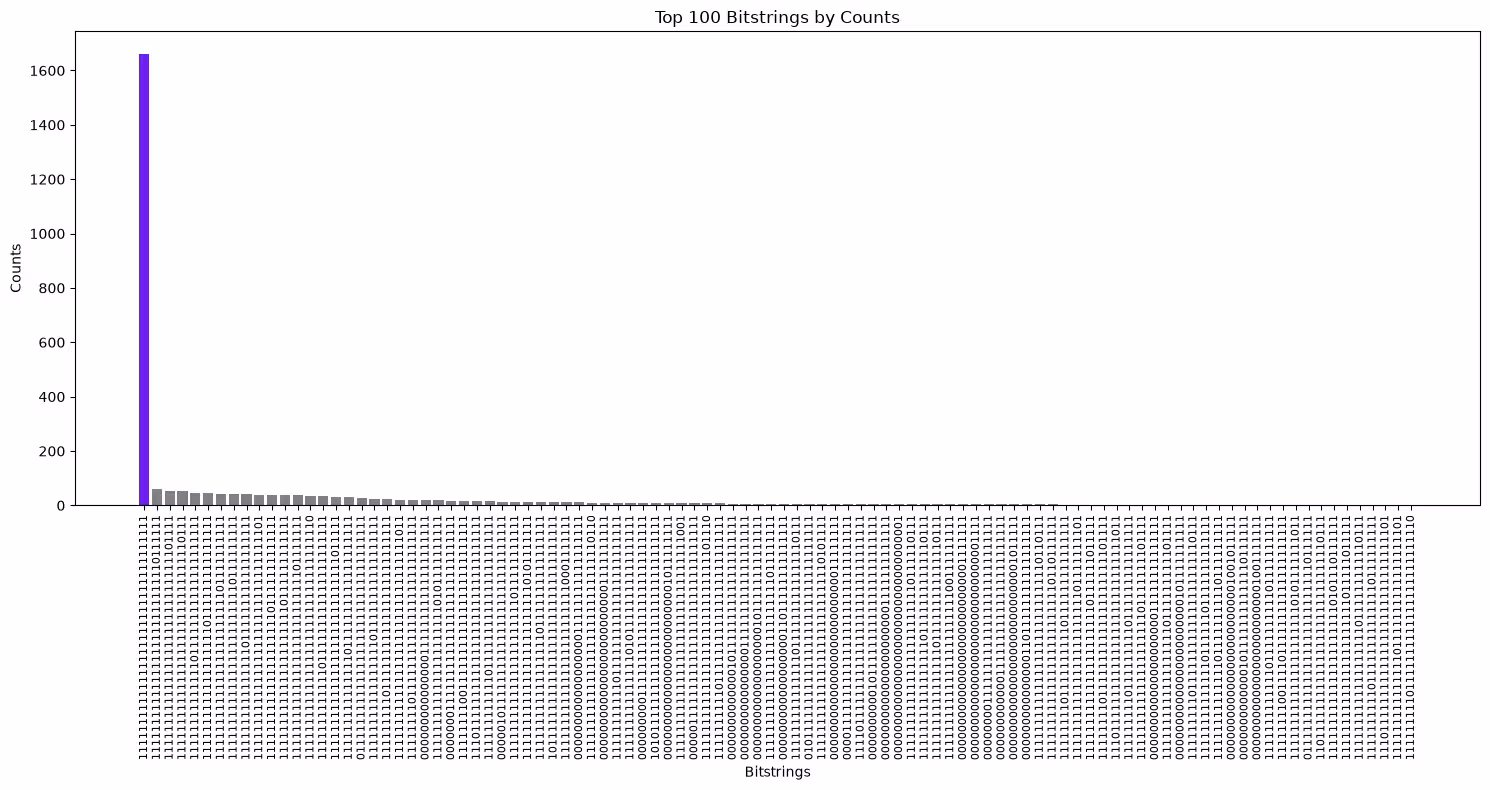
3. Plot the top bitstrings

Plot the bitstring with the highest counts to see if the hidden bitstring was the mode.

import matplotlib.pyplot as plt


def plot_top_bitstrings(counts_dict, hidden_bitstring=None):
    # Sort and take the top 100 bitstrings
    top_100 = sorted(counts_dict.items(), key=lambda x: x[1], reverse=True)[
        :100
    ]
    if not top_100:
        print("No bitstrings found in the input dictionary.")
        return

    # Unzip the bitstrings and their counts
    bitstrings, counts = zip(*top_100)

    # Assign colors: purple if the bitstring matches hidden_bitstring, otherwise gray
    colors = [
        "#680CE9" if bit == hidden_bitstring else "gray" for bit in bitstrings
    ]

    # Create the bar plot
    plt.figure(figsize=(15, 8))
    plt.bar(
        range(len(bitstrings)), counts, tick_label=bitstrings, color=colors
    )

    # Rotate the bitstrings for better readability
    plt.xticks(rotation=90, fontsize=8)
    plt.xlabel("Bitstrings")
    plt.ylabel("Counts")
    plt.title("Top 100 Bitstrings by Counts")

    # Show the plot
    plt.tight_layout()
    plt.show()

The hidden bitstring is highlighted in purple, and it should be the bitstring with the highest number of counts.

plot_top_bitstrings(counts, hidden_bitstring)

Output:

Changelog

2026-02-20: Deprecation Notice - the provider_job_ids metadata field will be deprecated in 30 days in version 0.13.0. Users can access the job ID through job_id() method of the runtime service.
2026-02-11: We now have support for ibm_miami, and added execution metadata to the PubResult.

Get support

For any questions or issues, contact Q-CTRL.

Next steps

Recommendations