Singularity Machine Learning - Classification: A Qiskit Function by Multiverse Computing
See the API reference
The code on this page was developed using the following requirements. We recommend using these versions or newer.
scikit-learn~=1.8.0
- Qiskit Functions are an experimental feature available only to IBM Quantum® Premium Plan, Flex Plan, and On-Prem (via IBM Quantum Platform API) Plan users. They are in preview release status and subject to change.
Overview
With the "Singularity Machine Learning - Classification" function, you can solve real-world machine learning problems on quantum hardware without requiring quantum expertise. This Application function, based on ensemble methods, is a hybrid classifier. It leverages classical methods like boosting, bagging, and stacking for initial ensemble training. Subsequently, quantum algorithms such as variational quantum eigensolver (VQE) and quantum approximate optimization algorithm (QAOA) are employed to enhance the trained ensemble's diversity, generalization capabilities, and overall complexity.
Unlike other quantum machine learning solutions, this function is capable of handling large-scale datasets with millions of examples and features without being limited by the number of qubits in the target QPU. The number of qubits only determines the size of the ensemble that can be trained. It is also highly flexible, and can be used to solve classification problems across a wide range of domains, including finance, healthcare, and cybersecurity.
It consistently achieves high accuracies on classically challenging problems involving high-dimensional, noisy, and imbalanced datasets.
It is built for:
- Engineers and data scientists at companies seeking to enhance their tech offerings by integrating quantum machine learning into their products and services,
- Researchers at quantum research labs exploring quantum machine learning applications and looking to leverage quantum computing for classification tasks, and
- Students and teachers at educational institutions in courses like machine learning, and who are looking to demonstrate the advantages of quantum computing.
The following example showcases its various functionalities, including create, list, fit, and predict, and demonstrates its usage in a synthetic problem comprising two interleaving half circles, a notoriously challenging problem due to its nonlinear decision boundary.
Function description
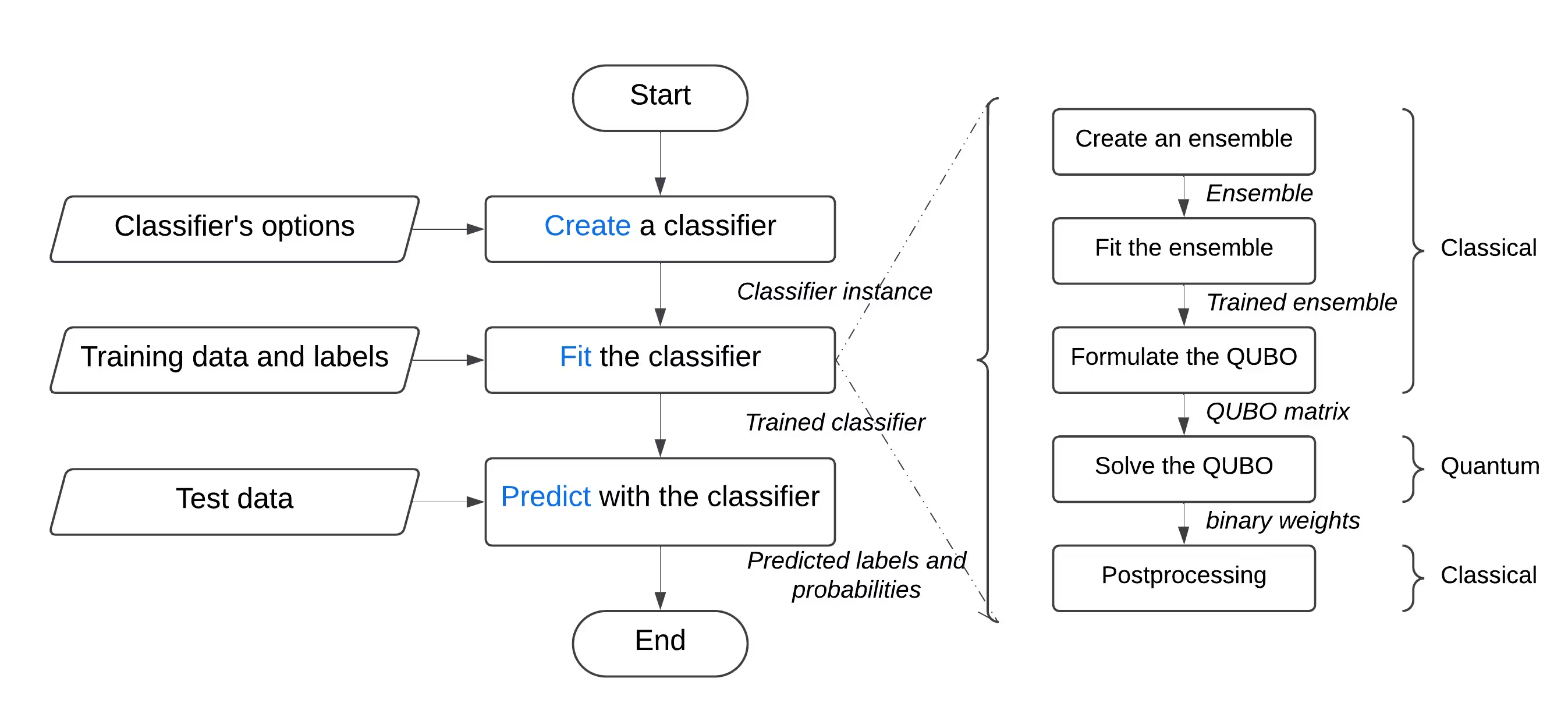
This Qiskit Function allows users to solve binary classification problems using Singularity's quantum-enhanced ensemble classifier. Behind the scenes, it uses a hybrid approach to classically train an ensemble of classifiers on the labeled dataset, and then optimize it for maximum diversity and generalization using the Quantum Approximate Optimization Algorithm (QAOA) on IBM® QPUs. Through a user-friendly interface, users can configure a classifier according to their requirements, train it on the dataset of their choice, and use it to make predictions on a previously unseen dataset.
To solve a generic classification problem:
- Preprocess the dataset, and split it into training and testing sets. Optionally, you can further split the training set into training and validation sets. This can be achieved using scikit-learn.
- If the training set is imbalanced, you can resample it to balance the classes using imbalanced-learn.
- Upload the training, validation, and test sets separately to the function's storage using the catalog's
file_uploadmethod, passing it the relevant path each time. - Initialize the quantum classifier by using the function's
createaction, which accepts hyperparameters such as the number and types of learners, the regularization (lambda value), and optimization options including the number of layers, the type of classical optimizer, the quantum backend, and so on. - Train the quantum classifier on the training set using the function's
fitaction, passing it the labeled training set, and the validation set if applicable. - Make predictions on the previously unseen test set using the function's
predictaction.
Get started
Authenticate using your IBM Quantum Platform API key, and select the Qiskit Function as follows:
from qiskit_ibm_catalog import QiskitFunctionsCatalog

catalog = QiskitFunctionsCatalog(channel="ibm_quantum_platform")

# Verify that you have access to the function
catalog.list()
Output:
[QiskitFunction(qunova/hivqe-chemistry),
 QiskitFunction(global-data-quantum/quantum-portfolio-optimizer),
 QiskitFunction(algorithmiq/tem),
 QiskitFunction(qedma/qesem),
 QiskitFunction(multiverse/singularity),
 QiskitFunction(ibm/circuit-function),
 QiskitFunction(q-ctrl/optimization-solver),
 QiskitFunction(colibritd/quick-pde),
 QiskitFunction(q-ctrl/performance-management),
 QiskitFunction(kipu-quantum/iskay-quantum-optimizer)]
# load function
singularity = catalog.load("multiverse/singularity")
Examples
Classify a dataset
In this example, you'll use the "Singularity Machine Learning - Classification" function to classify a dataset consisting of two interleaving, moon-shaped half-circles. The dataset is synthetic, two-dimensional, and labeled with binary labels. It is created to be challenging for algorithms such as centroid-based clustering and linear classification.

Through this process, you'll learn how to create the classifier, fit it to the training data, use it to predict on the test data, and delete the classifier when you're finished.
Before starting, you need to install scikit-learn. Install it using the following command:
python3 -m pip install scikit-learnPerform the following steps:
- Create the synthetic dataset using the
make_moonsfunction from scikit-learn. - Upload the generated synthetic dataset to the shared data directory.
- Create the quantum-enhanced classifier using the
createaction. - Enlist your classifiers using the
listaction. - Train the classifier on the train data using the
fitaction. - Use the trained classifier to predict on the test data using the
predictaction. - Delete the classifier using the
deleteaction. - Clean up after you're done.
Step 1. Import the necessary modules and generate the synthetic dataset, then split it into training and test datasets.
# import the necessary modules for this example
import os
import tarfile
import numpy as np

# Import the make_moons and the train_test_split functions from scikit-learn
# to create a synthetic dataset and split it into training and test datasets
from sklearn.datasets import make_moons
from sklearn.model_selection import train_test_split

# generate the synthetic dataset
X, y = make_moons(n_samples=10000)

# split the data into training and test datasets
X_train, X_test, y_train, y_test = train_test_split(X, y, test_size=0.2)

# print the first 10 samples of the training dataset
print("Features:", X_train[:10, :])
print("Targets:", y_train[:10])
Output:
Features: [[ 0.84757037 -0.48831433]
 [ 0.98132552  0.19235443]
 [-0.71626723  0.6978261 ]
 [ 1.18957848 -0.48186557]
 [ 0.52118982 -0.37791846]
 [ 0.81115408  0.58483251]
 [ 0.48706462  0.87336593]
 [-0.81880144  0.57407682]
 [ 1.67335408 -0.23932015]
 [ 0.50181306  0.8649761 ]]
Targets: [1 0 0 1 1 0 0 0 1 0]
Step 2. Save the labeled training and test datasets on your local disk, and then upload them to the shared data directory.
def make_tarfile(file_path, tar_file_name):
    with tarfile.open(tar_file_name, "w") as tar:
        tar.add(file_path, arcname=os.path.basename(file_path))


# save the training and test datasets on your local disk
np.save("X_train.npy", X_train)
np.save("y_train.npy", y_train)
np.save("X_test.npy", X_test)
np.save("y_test.npy", y_test)

# create tar files for the datasets
make_tarfile("X_train.npy", "X_train.npy.tar")
make_tarfile("y_train.npy", "y_train.npy.tar")
make_tarfile("X_test.npy", "X_test.npy.tar")
make_tarfile("y_test.npy", "y_test.npy.tar")

# upload the datasets to the shared data directory
catalog.file_upload("X_train.npy.tar", singularity)
catalog.file_upload("y_train.npy.tar", singularity)
catalog.file_upload("X_test.npy.tar", singularity)
catalog.file_upload("y_test.npy.tar", singularity)

# view/enlist the uploaded files in the shared data directory
print(catalog.files(singularity))
Output:
['X_test.npy.tar', 'X_train.npy.tar', 'y_test.npy.tar', 'y_train.npy.tar']
Step 3. Create a quantum-enhanced classifier using the create action.
job = singularity.run(
    action="create",
    name="my_classifier",
    num_learners=10,
    learners_types=[
        "DecisionTreeClassifier",
        "KNeighborsClassifier",
    ],
    learners_proportions=[0.5, 0.5],
    learners_options=[{}, {}],
    regularization=0.01,
    weight_update_method="logarithmic",
    sample_scaling=True,
    optimizer_options={"simulator": True},
    voting="soft",
    prob_threshold=0.5,
)

print(job.result())
Output:
{'status': 'ok', 'message': 'Classifier created.', 'data': {}, 'metadata': {'resource_usage': {}}}
# list available classifiers using the list action
job = singularity.run(action="list")

print(job.result())

# you can also find your classifiers in the shared data directory with a *.pkl.tar extension
print(catalog.files(singularity))
Output:
{'status': 'ok', 'message': 'Classifiers listed.', 'data': {'classifiers': ['my_classifier']}, 'metadata': {'resource_usage': {}}}
['X_test.npy.tar', 'X_train.npy.tar', 'my_classifier.pkl.tar', 'y_test.npy.tar', 'y_train.npy.tar']
Step 4. Train the quantum-enhanced classifier using the fit action.
job = singularity.run(
    action="fit",
    name="my_classifier",
    X="X_train.npy",  # you do not need to specify the tar extension
    y="y_train.npy",  # you do not need to specify the tar extension
)

print(job.result())
Output:
{'status': 'ok', 'message': 'Classifier fitted.', 'data': {}, 'metadata': {'resource_usage': {'RUNNING: MAPPING': {'CPU_TIME': 13.655871629714966}, 'RUNNING: WAITING_QPU': {'CPU_TIME': 54.688621282577515}, 'RUNNING: POST_PROCESSING': {'CPU_TIME': 56.92286920547485}, 'RUNNING: EXECUTING_QPU': {'QPU_TIME': 57.92738223075867}}}}
Step 5. Obtain predictions and probabilities from the quantum-enhanced classifier using the predict action.
job = singularity.run(
    action="predict",
    name="my_classifier",
    X="X_test.npy",  # you do not need to specify the tar extension
)

result = job.result()

print("Action result status: ", result["status"])
print("Action result message: ", result["message"])
print("Predictions (first five results):", result["data"]["predictions"][:5])
print(
    "Probabilities (first five results):", result["data"]["probabilities"][:5]
)
Output:
Action result status:  ok
Action result message:  Classifier predicted.
Predictions (first five results): [0, 0, 1, 0, 1]
Probabilities (first five results): [[1.0, 0.0], [1.0, 0.0], [0.0, 1.0], [1.0, 0.0], [0.0, 1.0]]
Step 6. Delete the quantum-enhanced classifier using the delete action.
job = singularity.run(
    action="delete",
    name="my_classifier",
)

# or you can delete from the shared data directory
# catalog.file_delete("my_classifier.pkl.tar", singularity)

print(job.result())
Output:
{'status': 'ok', 'message': 'Classifier deleted.', 'data': {}, 'metadata': {'resource_usage': {}}}
Step 7. Clean up local and shared data directories.
# delete the numpy files from your local disk
os.remove("X_train.npy")
os.remove("y_train.npy")
os.remove("X_test.npy")
os.remove("y_test.npy")

# delete the tar files from your local disk
os.remove("X_train.npy.tar")
os.remove("y_train.npy.tar")
os.remove("X_test.npy.tar")
os.remove("y_test.npy.tar")

# delete the tar files from the shared data
catalog.file_delete("X_train.npy.tar", singularity)
catalog.file_delete("y_train.npy.tar", singularity)
catalog.file_delete("X_test.npy.tar", singularity)
catalog.file_delete("y_test.npy.tar", singularity)
Output:
'Requested file was deleted.'
create_fit_predict example
The following example demonstrates the create_fit_predict action.
# Import QiskitFunctionsCatalog to load the
# "Singularity Machine Learning - Classification" function by Multiverse Computing
from qiskit_ibm_catalog import QiskitFunctionsCatalog

# Import the make_moons and the train_test_split functions from scikit-learn
# to create a synthetic dataset and split it into training and test datasets
from sklearn.datasets import make_moons
from sklearn.model_selection import train_test_split

# authentication
# If you have not previously saved your credentials, follow instructions at
# /docs/guides/functions
# to authenticate with your API key.
catalog = QiskitFunctionsCatalog(channel="ibm_quantum_platform")

# load "Singularity Machine Learning - Classification" function by Multiverse Computing
singularity = catalog.load("multiverse/singularity")

# generate the synthetic dataset
X, y = make_moons(n_samples=1000)

# split the data into training and test datasets
X_train, X_test, y_train, y_test = train_test_split(X, y, test_size=0.2)

job = singularity.run(
    action="create_fit_predict",
    num_learners=10,
    regularization=0.01,
    optimizer_options={"simulator": True},
    X_train=X_train,
    y_train=y_train,
    X_test=X_test,
    options={"save": False},
)

# get job status and result
status = job.status()
result = job.result()

print("Job status: ", status)
print("Action result status: ", result["status"])
print("Action result message: ", result["message"])
print("Predictions (first five results): ", result["data"]["predictions"][:5])
print(
    "Probabilities (first five results): ",
    result["data"]["probabilities"][:5],
)
print("Usage metadata: ", result["metadata"]["resource_usage"])
Output:
Job status:  QUEUED
Action result status:  ok
Action result message:  Classifier created, fitted, and predicted.
Predictions (first five results):  [0, 0, 1, 0, 0]
Probabilities (first five results):  [[0.87119766531518, 0.1288023346848197], [0.87119766531518, 0.1288023346848197], [0.24470328446479797, 0.7552967155352032], [0.820524432250189, 0.17947556774981072], [0.6847610293419495, 0.31523897065805173]]
Usage metadata:  {'RUNNING: MAPPING': {'CPU_TIME': 10.967791318893433}, 'RUNNING: WAITING_QPU': {'CPU_TIME': 59.91712307929993}, 'RUNNING: POST_PROCESSING': {'CPU_TIME': 59.097386837005615}, 'RUNNING: EXECUTING_QPU': {'QPU_TIME': 56.93338203430176}}
Benchmarks
These benchmarks show that the classifier can achieve extremely high accuracies on challenging problems. They also show that increasing the number of learners in the ensemble (number of qubits) can lead to increased accuracy.
"Classical accuracy" refers to the accuracy obtained using corresponding classical state of the art which, in this case, is an AdaBoost classifier based on an ensemble of size 75. "Quantum accuracy", on the other hand, refers to the accuracy obtained using the "Singularity Machine Learning - Classification".
Problem | Dataset Size | Ensemble Size | Number of Qubits | Classical Accuracy | Quantum Accuracy | Improvement |
|---|---|---|---|---|---|---|
| Grid stability | 5000 examples, 12 features | 55 | 55 | 76% | 91% | 15% |
| Grid stability | 5000 examples, 12 features | 65 | 65 | 76% | 92% | 16% |
| Grid stability | 5000 examples, 12 features | 75 | 75 | 76% | 94% | 18% |
| Grid stability | 5000 examples, 12 features | 85 | 85 | 76% | 94% | 18% |
| Grid stability | 5000 examples, 12 features | 100 | 100 | 76% | 95% | 19% |
As quantum hardware evolves and scales, the implications for our quantum classifier become increasingly significant. While the number of qubits does impose limitations on the size of the ensemble that can be utilized, it does not restrict the volume of data that can be processed. This powerful capability enables the classifier to efficiently handle datasets containing millions of data points and thousands of features. Importantly, the constraints related to ensemble size can be addressed through the implementation of a large-scale version of the classifier. By leveraging an iterative outer-loop approach, the ensemble can be dynamically expanded, enhancing flexibility and overall performance. However, it's worth noting that this feature has not yet been implemented in the current version of the classifier.
Changelog
4 June 2025
- Upgraded
QuantumEnhancedEnsembleClassifierwith the following updates:- Added onsite/alpha regularization. You can specify
regularization_typeto beonsiteoralpha - Added auto-regularization. You can set
regularizationtoautoto use auto-regularization - Added
optimization_dataparameter to thefitmethod to choose optimization data for quantum optimization. You can use one of these options:train,validation, orboth - Improved overall performance
- Added onsite/alpha regularization. You can specify
- Added detailed status tracking for running jobs
20 May 2025
- Standardized error handling
18 March 2025
- Upgraded qiskit-serverless to 0.20.0 and base image to 0.20.1
14 February 2025
- Upgraded base image to 0.19.1
6 February 2025
- Upgraded qiskit-serverless to 0.19.0 and base image to 0.19.0
13 November 2024
- Release of Singularity Machine Learning - Classification
Get support
For any questions, reach out to Multiverse Computing.
Be sure to include the following information:
- The Qiskit Function Job ID (
job.job_id) - A detailed description of the issue
- Any relevant error messages or codes
- Steps to reproduce the issue
Next steps
- Request access to Multiverse Computing's Singularity Machine Learning Classification function.
- Visit the API reference for this Qiskit Function.
- Review Leclerc, L., et al. (2023). Financial risk management on a neutral atom quantum processor. Physical Review Research, 5, 043117.