Quantum Portfolio Optimizer: A Qiskit Function by Global Data Quantum
See the API reference
Qiskit Functions are an experimental feature available only to IBM Quantum® Premium Plan, Flex Plan, and On-Prem (via IBM Quantum Platform API) Plan users. They are in preview release status and subject to change.
Overview
The Quantum Portfolio Optimizer is a Qiskit Function that tackles the dynamic portfolio optimization problem, a standard problem in finance that aims to rebalance periodic investments across a set of assets, to maximize returns and minimize risks. By deploying cutting-edge quantum optimization techniques, this function simplifies the process so that users, with no expertise in quantum computing, can benefit from its advantages in finding optimal investment trajectories. Ideal for portfolio managers, researchers in quantitative finance, and individual investors, this tool enables back-testing of trading strategies in portfolio optimization.
Function description
The Quantum Portfolio Optimizer function uses the Variational Quantum Eigensolver (VQE) algorithm to solve a Quadratic Unconstrained Binary Optimization (QUBO) problem, addressing dynamic portfolio optimization problems. Users simply need to provide the asset price data and define the investment constraint, then the function runs the quantum optimization process that returns a set of optimized investment trajectories.
The process consists of four main stages. First, the input data is mapped to a quantum-compatible problem, constructing the QUBO of the dynamic portfolio optimization problem, and transforming it into a quantum operator (Ising Hamiltonian). Next, the input problem and the VQE algorithm are adapted to be run in the quantum hardware. The VQE algorithm is then run on the quantum hardware, and finally, the results are post-processed to provide the optimal investment trajectories. The system also includes a noise-aware (SQD-based) post-processing to maximize the quality of the output.
This Qiskit Function is based on the published manuscript by Global Data Quantum.


Get started
Authenticate using your API key and select the Qiskit Function as follows. (This snippet assumes you've already saved your account to your local environment.)
from qiskit_ibm_catalog import QiskitFunctionsCatalog

catalog = QiskitFunctionsCatalog(channel="ibm_quantum_platform")

# Verify that you have access to the function
catalog.list()
Output:
[QiskitFunction(qunova/hivqe-chemistry),
 QiskitFunction(global-data-quantum/quantum-portfolio-optimizer),
 QiskitFunction(algorithmiq/tem),
 QiskitFunction(qedma/qesem),
 QiskitFunction(multiverse/singularity),
 QiskitFunction(ibm/circuit-function),
 QiskitFunction(q-ctrl/optimization-solver),
 QiskitFunction(colibritd/quick-pde),
 QiskitFunction(q-ctrl/performance-management),
 QiskitFunction(kipu-quantum/iskay-quantum-optimizer)]
# Access function
dpo_solver = catalog.load("global-data-quantum/quantum-portfolio-optimizer")
Example: Dynamic portfolio optimization with seven assets
This example demonstrates how to execute the dynamic portfolio optimization (DPO) function and adjust its settings for optimal performance. It includes detailed steps for fine-tuning the parameters to achieve the desired outcomes.
This case involves seven assets, four time steps, and four resolution qubits, resulting in a total requirement of 112 qubits.
1. Read the assets included in the portfolio
If all the assets in the portfolio are stored in a folder at a specific path, you can load them into a pandas.DataFrame and convert it to a dict format object using the following function.
import os
import glob
import pandas as pd
def read_and_join_csv(file_pattern):
"""
Reads multiple CSV files matching the file pattern and combines them
into a single DataFrame.
Parameters:
file_pattern (str): The pattern to match CSV files.
Returns:
pd.DataFrame: Combined DataFrame with data from all CSV files.
"""
# Find all files matching the pattern
csv_files = glob.glob(file_pattern)
# Get the base file names without the .csv extension
file_names = [os.path.basename(f).replace(".csv", "") for f in csv_files]
# Read each CSV file into a DataFrame and set the first column as the index
df_list = [pd.read_csv(f).set_index("Unnamed: 0") for f in csv_files]
# Rename columns in each DataFrame to the base file names
for df, name in zip(df_list, file_names):
df.columns = [name]
# Combine all DataFrames into one by merging them side by side
combined_df = pd.concat(df_list, axis=1)
return combined_df
file_pattern = "route/to/folder/with/assets/data/*.csv"
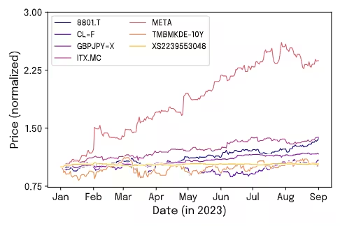
assets = read_and_join_csv(file_pattern).to_dict()For this example, we have used the assets 8801.T, CLF, GBPJPY, ITX.MC, META, TMBMKDE-10Y, and XS2239553048. The following figure illustrates the data used in this example, showing the daily closing price evolution of the assets from 1 January to 1 September in 2023.
In this example, to ensure uniformity across dates, we have filled non-trading days with the closing price from the previous available date. We apply this step because the selected assets come from different markets with varying trading days, making it essential to standardize the dataset for consistency.
2. Define the problem
Define the specifications of the problem by configuring the parameters in the qubo_settings dictionary.
qubo_settings = {
    "nt": 4,
    "nq": 4,
    "dt": 30,
    "max_investment": 25,
    "risk_aversion": 1000.0,
    "transaction_fee": 0.01,
    "restriction_coeff": 1.0,
}
3. Define the optimizer and ansatz settings (Optional)
Optionally define specific requirements for the optimization process, including the selection of the optimizer and its parameters, as well as the specification of the primitive and its configurations.
For the Tailored Ansatz, the chosen population size was based on previous experiments showing that this value yields stable and efficient optimization.
In the case of the Real Amplitudes Ansatz, you can follow a linear relationship between the population_size and the number of qubits in the circuit. As an approximated rule of thumb, it is recommended to use a minimum population_size ~ 0.8 * n_qubits for the real_amplitudes ansatz.
It is expected that the Optimized Real Amplitudes will have a better optimization performance than the Real Amplitudes ansatz. However, the number of variables to optimize in this ansatz increases much faster than in the Real Amplitudes case (see the manuscript). Thus, for large problems, the Optimized Real Amplitudes requires more circuit executions. The Optimized Real Amplitudes is likely to be useful for problems requiring up to 100 qubits, but it is recommended to be mindful when setting the population_size parameters. As an example of this scale-up in population_size, the previous table shows that for an 84-qubit problem, the Optimize Real Amplitudes requires 120 population_size, while for a 56-qubit problem, a population_size of 40 is enough.
optimizer_settings = {
    "de_optimizer_settings": {
        "num_generations": 20,
        "population_size": 90,
        "recombination": 0.4,
        "max_parallel_jobs": 5,
        "max_batchsize": 4,
        "mutation_range": [0.0, 0.25],
    },
    "optimizer": "differential_evolution",
    "primitive_settings": {
        "estimator_shots": 25_000,
        "estimator_precision": None,
        "sampler_shots": 100_000,
    },
}
It is also possible to choose a specific ansatz. The following uses the 'Tailored' ansatz.
ansatz_settings = {
    "ansatz": "tailored",
    "multiple_passmanager": False,
}
4. Run the problem
dpo_job = dpo_solver.run(
    assets=assets,
    qubo_settings=qubo_settings,
    optimizer_settings=optimizer_settings,
    ansatz_settings=ansatz_settings,
    backend_name="<backend name>",
    previous_session_id=[],
    apply_postprocess=True,
)
5. Retrieve results
The function returns a dictionary with the investment trajectories ordered from lowest to highest according to their objective function value (see the Output section of the API reference). This set of results allows for the identification of the trajectory with the lowest cost and its corresponding investment evaluations. Additionally, it provides for the analysis of different trajectories, facilitating the selection of those that best align with specific needs or objectives. This flexibility ensures that choices can be tailored to suit a variety of preferences or scenarios.
Begin by presenting the resulting strategy that achieved the lowest objective cost found during the process.
# Get the results of the job
dpo_result = dpo_job.result()

# Show the solution strategy
dpo_result["result"]
Output:
{'time_step_0': {'8801.T': 0.11764705882352941,
  'ITX.MC': 0.20588235294117646,
  'META': 0.38235294117647056,
  'GBPJPY=X': 0.058823529411764705,
  'TMBMKDE-10Y': 0.0,
  'CLF': 0.058823529411764705,
  'XS2239553048': 0.17647058823529413},
 'time_step_1': {'8801.T': 0.11428571428571428,
  'ITX.MC': 0.14285714285714285,
  'META': 0.2,
  'GBPJPY=X': 0.02857142857142857,
  'TMBMKDE-10Y': 0.42857142857142855,
  'CLF': 0.0,
  'XS2239553048': 0.08571428571428572},
 'time_step_2': {'8801.T': 0.0,
  'ITX.MC': 0.09375,
  'META': 0.3125,
  'GBPJPY=X': 0.34375,
  'TMBMKDE-10Y': 0.0,
  'CLF': 0.0,
  'XS2239553048': 0.25},
 'time_step_3': {'8801.T': 0.3939393939393939,
  'ITX.MC': 0.09090909090909091,
  'META': 0.12121212121212122,
  'GBPJPY=X': 0.18181818181818182,
  'TMBMKDE-10Y': 0.0,
  'CLF': 0.0,
  'XS2239553048': 0.21212121212121213}}
Afterwards, using the metadata, you can access the results of all the sampled strategies. You can thereby further analyze the alternative trajectories returned by the optimizer. To do this, read the dictionary stored in dpo_result['metadata']['all_samples_metrics'], which contains not only additional information about the optimal strategy, but also details of the other candidate strategies evaluated during the optimization.
The following example shows how to read this information using pandas to extract key metrics associated with the optimal strategy. These include Restriction Deviation, Sharpe Ratio, and the corresponding investment return.
# Convert metadata to a DataFrame
df = pd.DataFrame(dpo_result["metadata"]["all_samples_metrics"])

# Find the minimum objective cost
min_cost = df["objective_costs"].min()
print(f"Minimum Objective Cost Found: {min_cost:.2f}")

# Extract the row with the lowest cost
best_row = df[df["objective_costs"] == min_cost].iloc[0]

# Display the results associated with the best solution
print("Best Solution:")
print(f"  - Restriction Deviation: {best_row['rest_breaches']}%")
print(f"  - Sharpe Ratio: {best_row['sharpe_ratios']:.2f}")
print(f"  - Return: {best_row['returns']}")
Output:
Minimum Objective Cost Found: -3.78
Best Solution:
  - Restriction Deviation: 40.0
  - Sharpe Ratio: 24.82
  - Return: 0.46
6. Performance analysis
Last, analyze the performance of your optimization application. Specifically, compare your results, obtained in the previous example, against a random baseline to assess the effectiveness of our approach. If the quantum algorithm demonstrably and consistently produces results with lower cost values, it indicates an effective optimization process.
The figure presents the probability distributions of the objective costs. To generate these distributions, take the list of objective costs from the function result and count the occurrences of each cost value (values rounded to the second decimal place). Then, update the count column accordingly by joining counts of identical rounded values. Note that, for better visual comparison, the occurrence counts have been normalized so that each distribution is displayed between 0 and 1.

As shown in the figure (blue solid line), the cost distribution for our Variational Quantum Eigensolver (post-processed with SQD) approach is sharply concentrated at lower objective cost values, indicating good optimization performance. In contrast, the noisy baseline exhibits a broader distribution, centered around higher cost values. The gray dashed vertical line represents the mean value of the random distribution, further highlighting the consistency of the function in returning optimized investment strategies. For an additional comparison, the black dashed line in the figure corresponds to the solution obtained with the Gurobi optimizer (free version). All these results are further explored in the benchmarks below for the "Mixed Assets" example evaluated with the "Tailored" ansatz.
Benchmarks
This function was tested under different configurations of resolution qubits, ansatz circuits, and groupings of assets from various sectors: a mix of different assets (Set 1), oil derivatives (Set 2), and IBEX35 (Set 3). See more details in the following table.
Set | Date | Assets |
|---|---|---|
| Set 1 | 01/01/2023 | 8801.T, CL=F, GBPJPY=X, ITX.MC, META, TMBMKDE-10Y, XS2239553048 |
| Set 2 | 01/06/2023 | CL=F, BZ=F, HO=F, NG=F, XOM, RB=F, 2222.SR |
| Set 3 | 01/11/2022 | ACS.MC, ITX.MC, FER.MC, ELE.MC, SCYR.MC, AENA.MC, AMS.MC |
Two key metrics were used to evaluate solution quality.
- The objective cost, which measures optimization efficiency by comparing the cost function value from each experiment with results from Gurobi (free version).
- The Sharpe ratio, which captures the risk-adjusted return of each portfolio, offering insight into the financial performance of the solutions.
Together, these metrics benchmark both computational and financial aspects of the quantum-generated portfolios.
Example | Qubits | Ansatz | Depth | Runtime Usage (s) | Total usage (s) | Objective cost | Sharpe | Gurobi objective cost | Gurobi Sharpe |
|---|---|---|---|---|---|---|---|---|---|
| Mixed Assets (Set 1, 4 time steps, 4-bit) | 112 | Tailored | 83 | 12735 | 13095 | -3.78 | 24.82 | -4.25 | 24.71 |
| Mixed Assets (Set 1,4 time steps, 4 time steps, 4-bit) | 112 | Real Amplitudes | 359 | 11739 | 11903 | -3.39 | 23.64 | -4.25 | 24.71 |
| Oil Derivatives (Set 2, 4 time steps, 3-bit) | 84 | Optimized Real Amplitudes | 78 | 6180 | 6350 | -3.73 | 19.13 | -4.19 | 21.71 |
| IBEX35 (Set 3, 4 time steps, 2-bit) | 56 | Optimized Real Amplitudes | 96 | 3314 | 3523 | -3.67 | 14.48 | -4.11 | 16.44 |
Results show that the quantum optimizer, with problem-specific ansatzes, effectively identifies efficient investment strategies across various portfolio types.
Below we detail both the population size and the number of generations specified in the optimizer_options dictionary. All other parameters were set to their default values.
Example | population_size | num_generations |
|---|---|---|
| Mixed Assets Portfolio | 90 | 20 |
| Mixed Assets Portfolio | 92 | 20 |
| Oil Derivatives Portfolio | 120 | 20 |
| IBEX35 Portfolio | 40 | 20 |
The number of generations was set to 20, as this value was found to be sufficient to reach convergence. Additionally, the default values for the optimizer's internal parameters were left unchanged, as they consistently provided good performance and are generally recommended by the literature and implementation guidelines.
Get support
If you need help, you can send an email to qpo.support@globaldataquantum.com. In your message, provide the function job ID.
Next steps
- Read the associated research paper.
-
- Visit the API reference for this Qiskit Function.
- Request access to the function by filling in this form.
- Try the Dynamic Portfolio Optimization tutorial.